Why Does Theory Matter in Computer Science? /

Why Does Theory Matter in Computer Science? (Part 4)

Set Functions, Supermodularity and the Densest Supermodular Set Problem

• May 22, 2025
• talks  
• notes  
• math  
• computer science  
• explainers  
• graph theory  
• algorithms  

This is the fourth installment in the written version of my talk about why I think theory matters in computer science. You can find part 3 here and the entire series is archived here.

Digression: Submodularity, Modularity, Supermodularity, and Set functions

In Part 3, we discussed the densest subgraph problem (DSP) and some algorithms for solving it. In this section, we’ll be looking at how we can generalize this problem and those algorithms to solve some other problems.

We’re going to go on a detour for a while now. This is the scary section. It was scary for me, and it’ll probably be scary for you too, but we’ve gotten this far together. This is the part of the talk where I will introduce some fancy new math I had to learn in order to understand how one might generalize iterative peeling to solve adjacent problems.

As a preview of where I’m going with this, it turns out that iterative peeling works because the densest subgraph problem is a special case of something called the “densest supermodular set problem”. (Don’t worry, I’m going to break down what that means; that’s what this whole section of the talk is about.) Rephrasing the DSP in terms of this “supermodularity theory” gives us a unifying framework that explains the differing “error rates” between peeling and iterative peeling and also gives us a way to maybe get solutions to some related problems for free. We’re going to be getting a glimpse of how theoretical concepts are used to extend existing solutions to problems to other contexts.

So we’re going to learn some new ideas here, and we’re going to make some older ones precise. I think for some of you, “examples” might be the only word you recognize, whereas for others, some of this may be vaguely familiar. Either way, that’s okay. This is your moment to freak out.

*deep breath*

Alright, time’s up. Let’s get started.

Set Functions

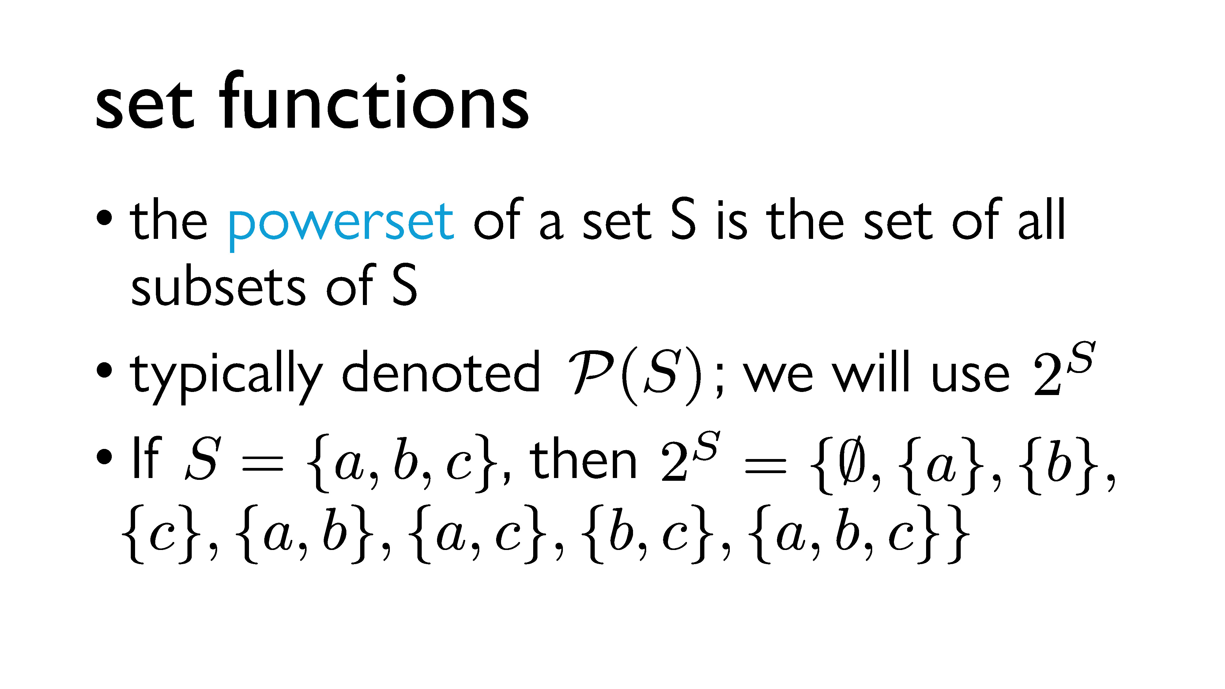
We’re going to kick off by talking about sets and set functions. As you likely remember from high school, a set $S$ is an unordered collection of distinct objects. The powerset of $S$ is the set of all subsets of $S$, which includes both the empty set (denoted ${}$ or $\emptyset$) and $S$ itself. Typically, this is denoted $\mathcal{P}(S)$, but we’re going to use this alternate $2^S$ notation¹, which is equivalent.

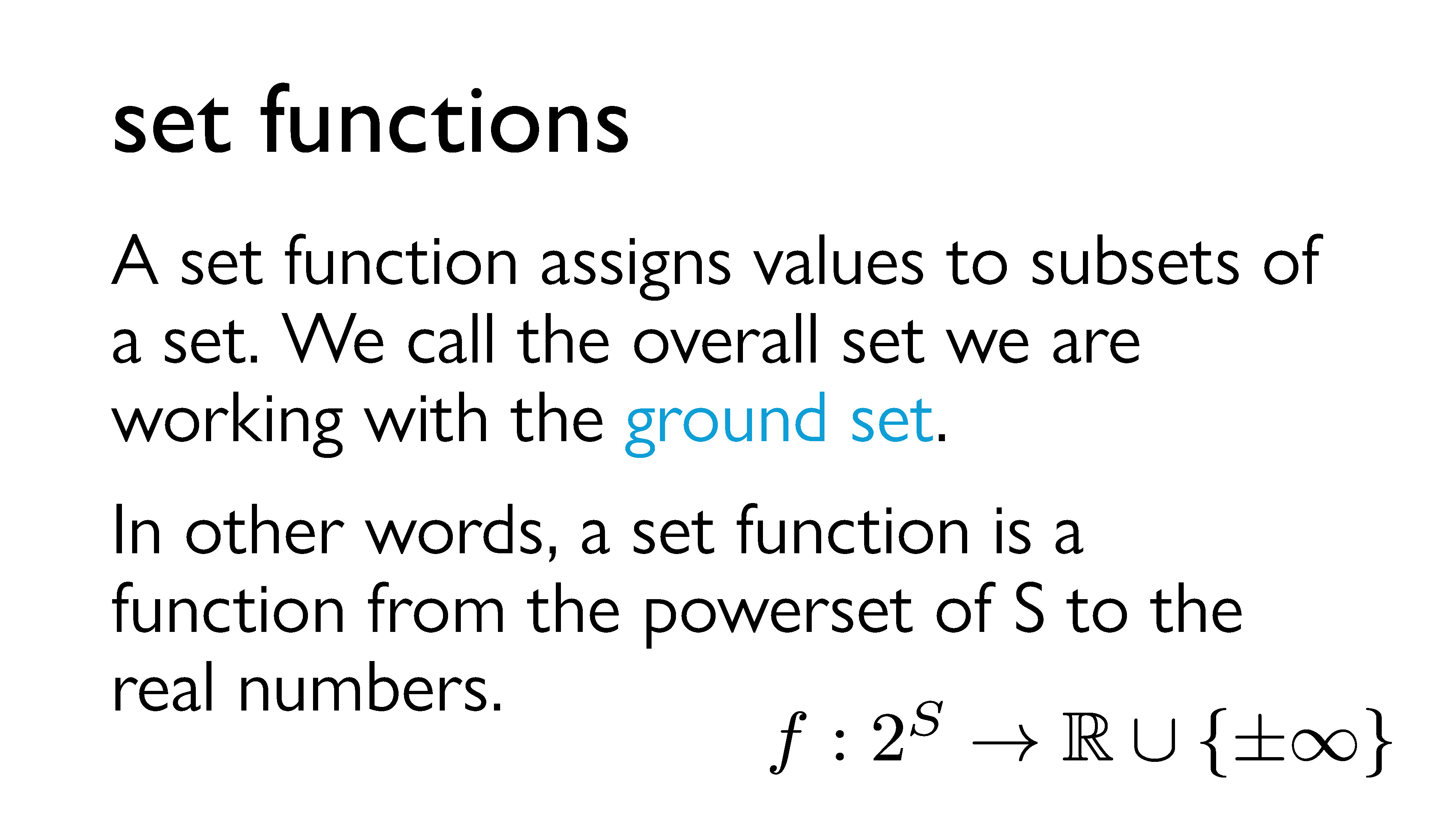
A set function $f: 2^S \rightarrow \mathbb{R}\cup {\pm\infty}$ is a special type of function that assigns a value to each subset of a set. First, a specific set we will be working with is defined, and we call that set the ground set. (This is $S$.) Then, we map every subset of the set to a real number (sometimes including positive and negative infinity). For example, if $S = \{a,b\}$, we might map $\emptyset$ to 0, $\{a\}$ to 1, $\{b\}$ to -2.5, and $\{a, b\}$ to 0.

In short, a set function is a function from the powerset of the ground set to the real numbers.

From this point on, we’re going to be using $S$ to mean some arbitrary subset, so we’re going to call our ground set $V$ instead. Here’s some useful terminology for different types of set functions.

Let $f : 2^V \rightarrow \mathbb{R}$. $f$ called:

• normalized if $f(\emptyset) = 0$
• monotone increasing if $A \subset B \implies f(A) < f(B)$
• monotone decreasing if $A \subset B \implies f(A) > f(B)$
• additive if $f(A ,\dot\cup, B) = f(A) + f(B)$ (that is, if for any disjoint sets $A$ and $B$, the union of $A$ and $B$ has a value equal to the sum of the values of $A$ and $B$)
• subadditive if $f(A ,\dot\cup, B) \leq f(A) + f(B)$
• superadditive if $f(A ,\dot\cup, B) \geq f(A) + f(B)$

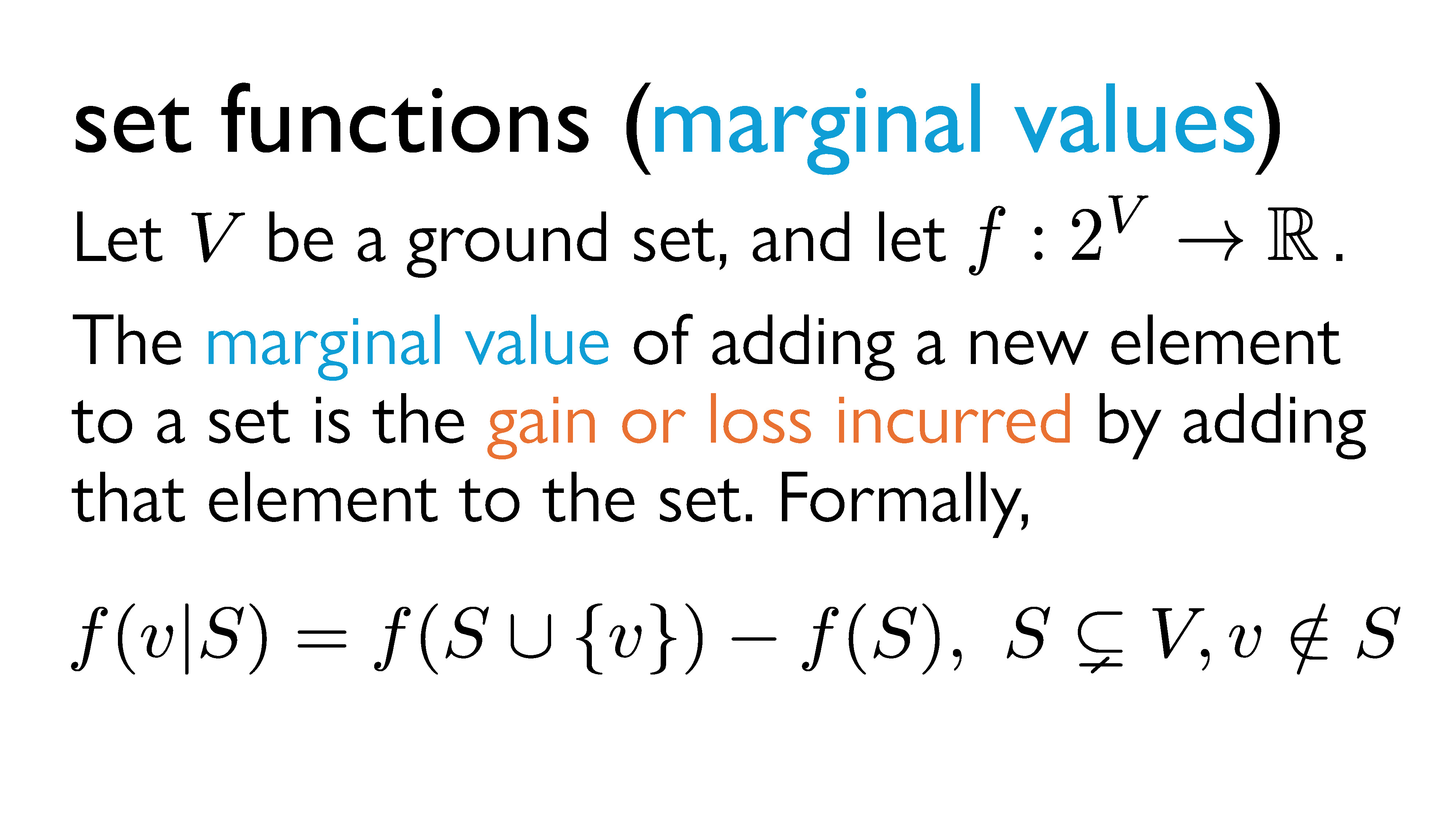
Another term that will be extremely useful for us is the concept of marginal values. The marginal value of adding a new element to a set is the gain or loss incurred by adding that element to the set. There are many equivalent notations for this, but we will denote this $f(v|S)$ (read “the marginal value of $v$ to $S$”).

Formally, for a set $S$ and an element $v$, $f(v|S) = f(S \cup \{v\}) - f(S)$, where $S \subsetneq V$ and $v \notin S$.

Marginal utility

Before I formally explain this modularity business, I want to take a brief interlude to explain a concept from economics that really helped these ideas make more concrete sense to me. This concept is called marginal utility. It refers to the extra value you get from having one additional unit of something. If we use pizza slices as an example, if you are very hungry, the first pizza slice you eat will have a very high value, because it will satiate your hunger. But subsequent pizza slices will have less value, because you won’t be as hungry anymore. If you eat too many slices, you might even feel sick, so that last slice would actually have negative value. So each slice of pizza you eat actually has diminishing returns, and most consumer goods follow something called the law of diminishing returns. However, diminishing marginal utility doesn’t apply in every scenario. For example, if we take bricks as an example, a single brick isn’t particularly useful on its own, and neither is a set of two or three bricks. However, a set of a million bricks is actually useful, because you can build something. So in the case of bricks, you actually get increasing returns with each new brick. (Well, not strictly – but this example is good enough for our purposes.)

Lastly, you can also have constant returns. For example, every single dollar has the same value. This means that every dollar you add to your bank account increases your purchasing power by the same amount.

We’ll formalize this notion a bit in a second, but abstractly, a submodular function is a set function characterized by diminishing returns. (You may be completely unsurprised to hear that economics really seem to like this concept.) A supermodular function is characterized by increasing returns, and a modular function is characterized by constant returns.

Submodular, Supermodular, and Modular Functions: Formal Definitions

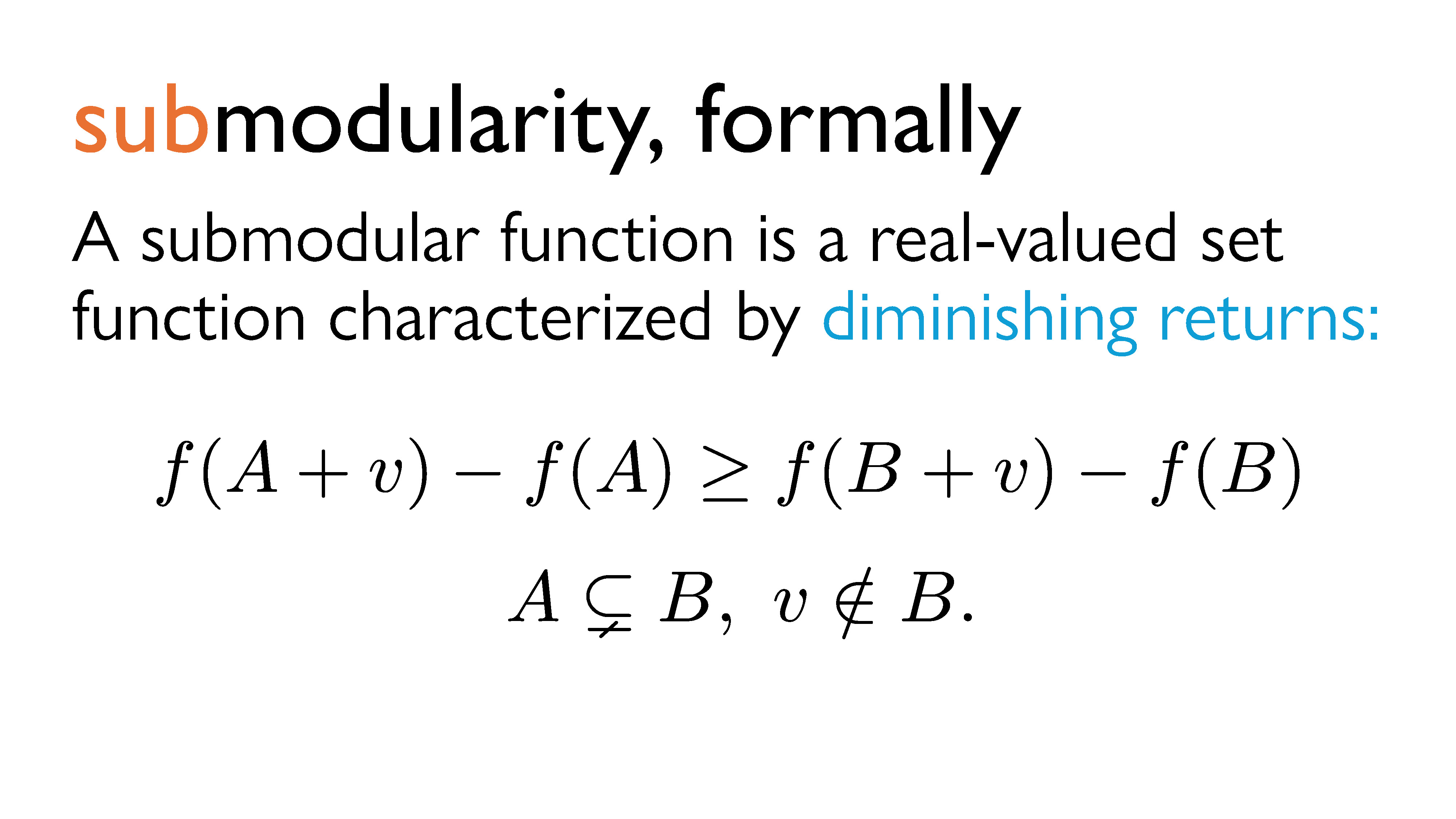
A submodular function is a real-valued set function characterized by diminishing returns. In other words, a very informal way to look at it is that the marginal value of $v$ to $S$ decreases as the number of elements in $S$ increases. Or, if $A$ is a (strict) subset of $B$, then adding $v$ to $A$ will induce a greater (or equal) change in value than adding $v$ to $B$.

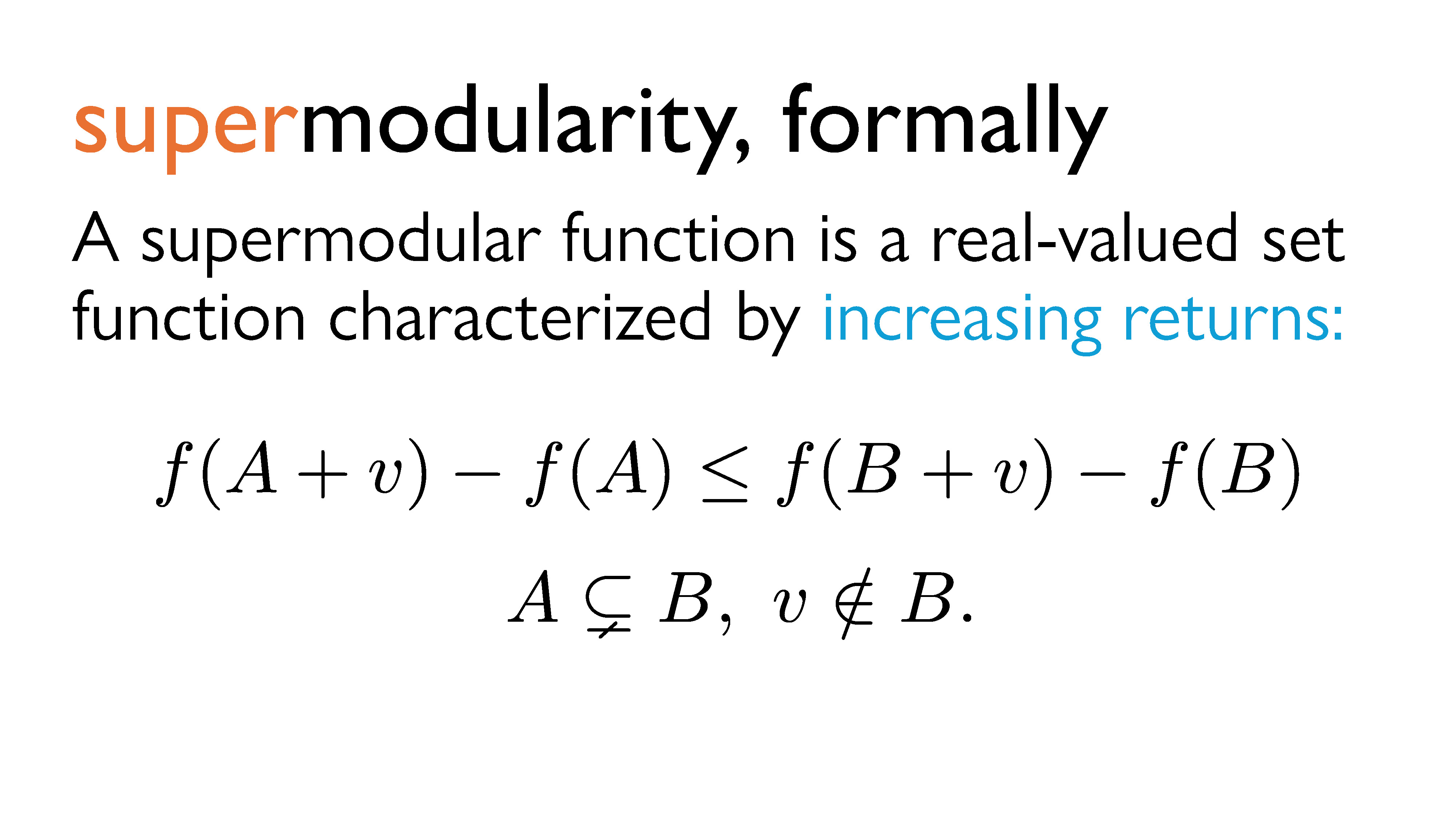
A supermodular function is a real-valued set function characterized by increasing returns. In other words, a very informal way to look at it is that the marginal value of $v$ to $S$ increases as the number of elements in $S$ increases. Or, if $A$ is a (strict) subset of $B$, then adding $v$ to $A$ will induce a lesser (or equal) change in value than adding $v$ to $B$.

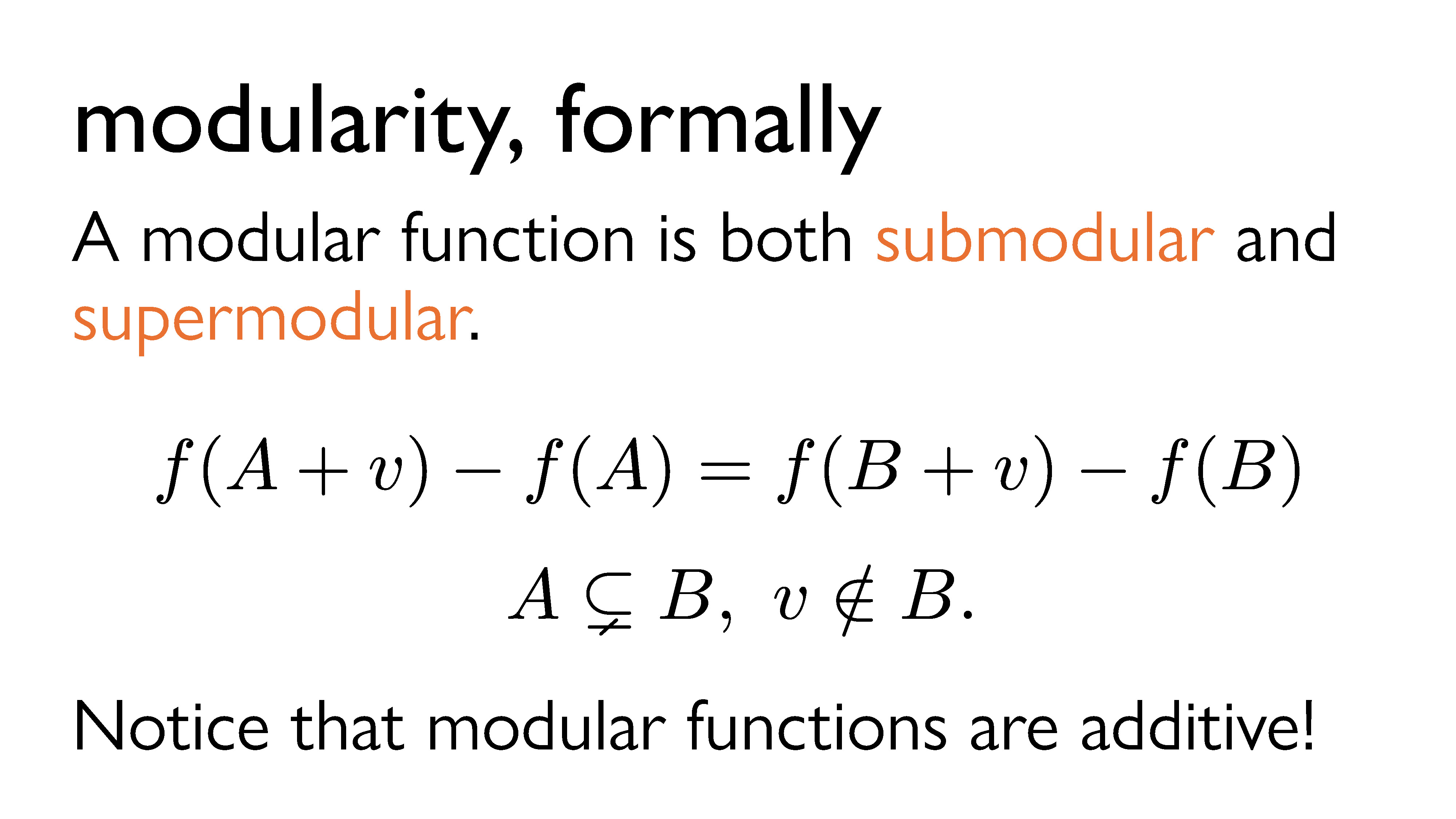
If a function is both submodular and supermodular, then we call it a modular function. Modular functions are characterized by constant returns. It’s worth noting that this implies that modular set functions are always additive.

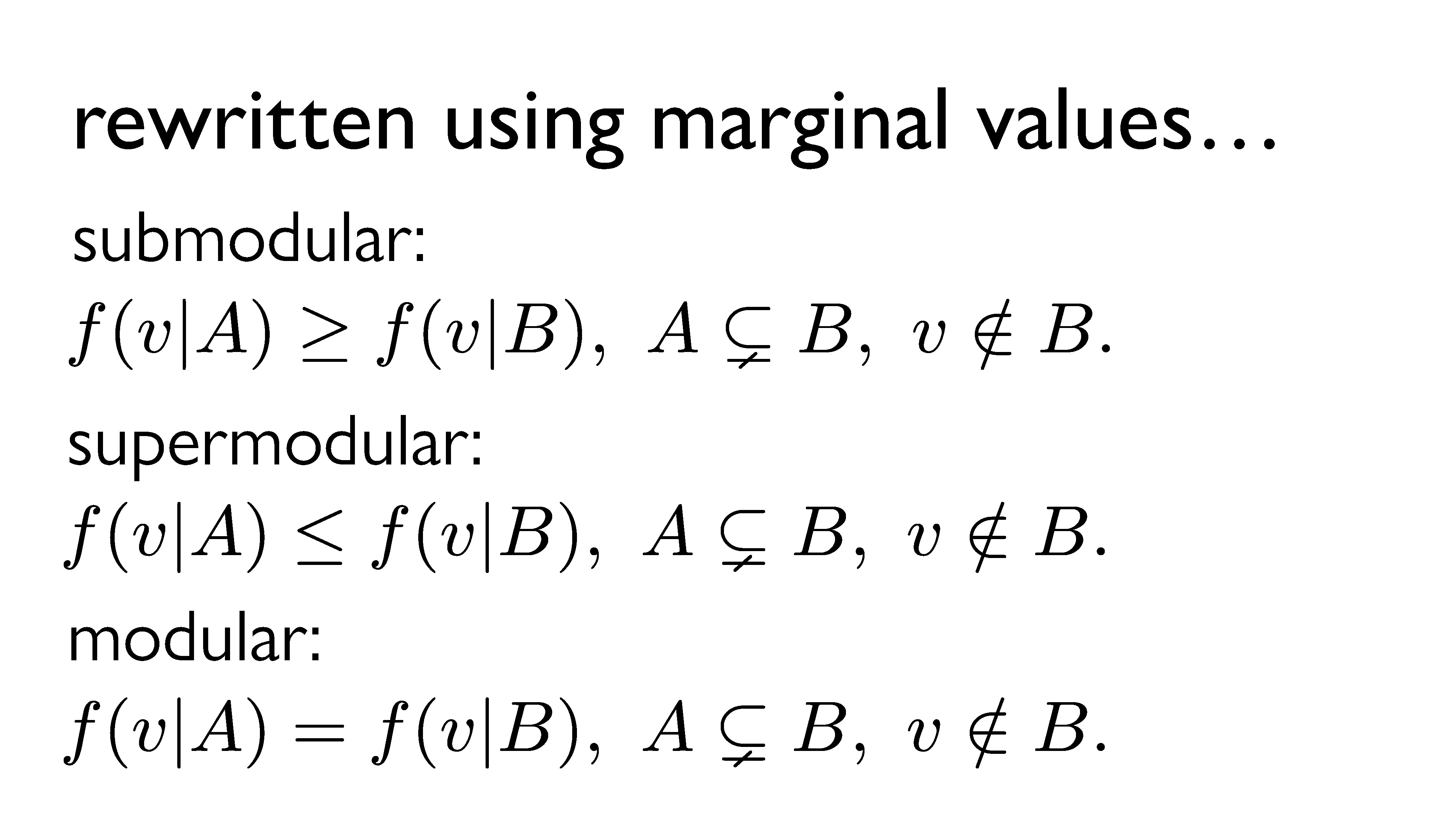
In summary, for $A \subsetneq B$, a set function $f$ is submodular if $f(v|A) \geq f(v|B)$, supermodular if $f(v|A) \leq f(v|B)$, and modular if $f(v|A) = f(v|B)$.

Generalization: The Densest Supermodular Set Problem (DSSP)

In part 3 of this talk, we discussed the densest subgraph problem (DSP) and some approximation algorithms for solving it. I then mentioned that by generalizing the problem even further, we might be able to solve some other problems. This generalization is known as the densest supermodular set problem (DSSP). First, we’ll take a look at what the DSSP actually is; then, we’ll discuss how it applies to both the DSP and potential related problems.

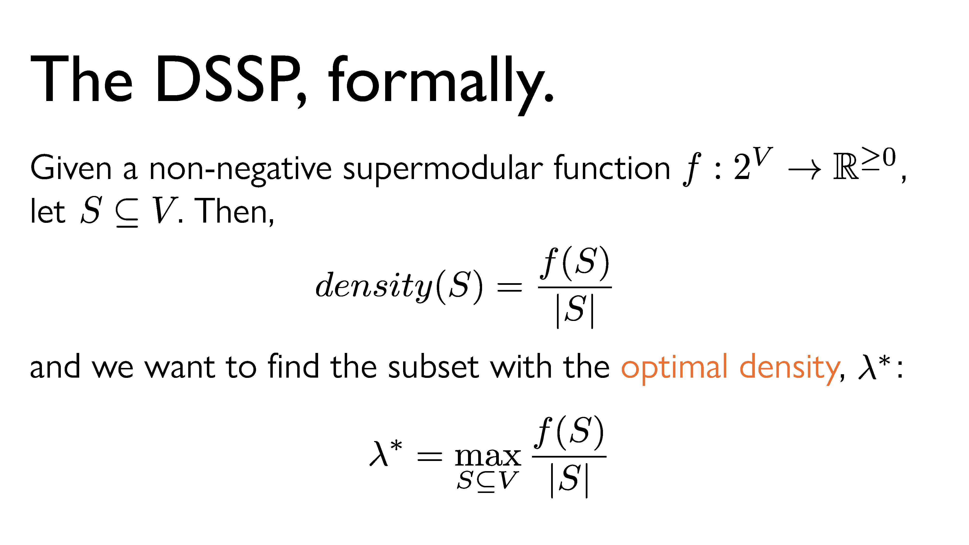
Here’s a somewhat formal statement of the DSSP. First, we define some ground set $V$, and a set function $f: 2^V \rightarrow \mathbb{R}^{\geq 0}$. For any subset $S$ of $V$, we define its density to be its value under $f$ divided by its size. That is, $density(S) = \frac{f(S)}{|S|}$. Now, we want to find the subset that maximizes the density. We’re going to call that density the the optimal density and denote it $\lambda^*$. Now, this might all sound very abstract. What’s up with all these sets? What is this supermodular function, and how can we use it to optimize anything? But remember, a supermodular function just assigns values to subsets in such a way that they exhibit the increasing returns property. As an example, it’s worth noting that our induced-edge counting function from earlier, $|E(S)|$, is actually supermodular. Let’s let $f = |E(S)|$, where $S$ is a set of vertices in a graph.

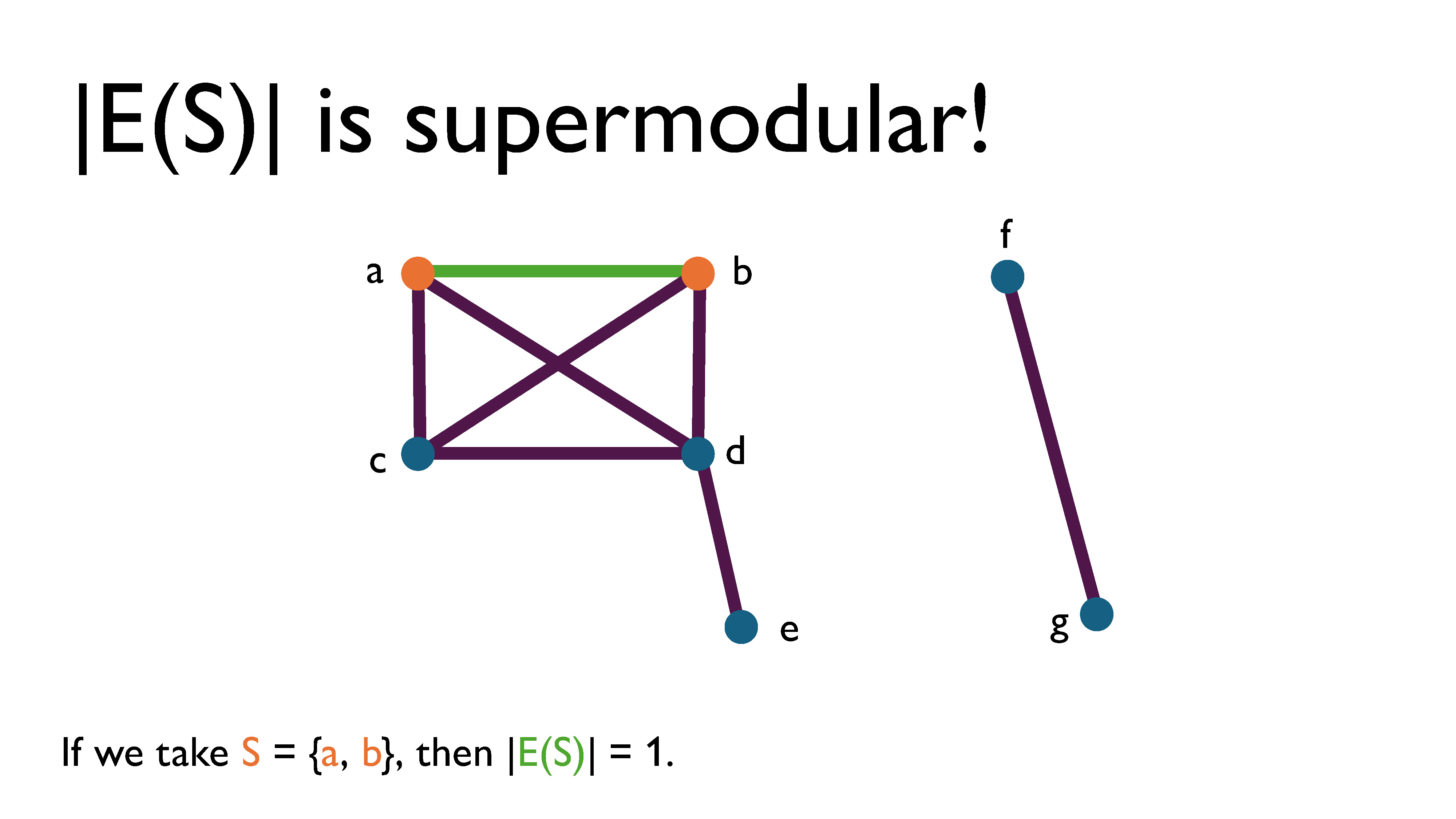
If we look at the example graph above, we see that if we take $S = \{a, b\}$, then $|E(S)| = 1$.

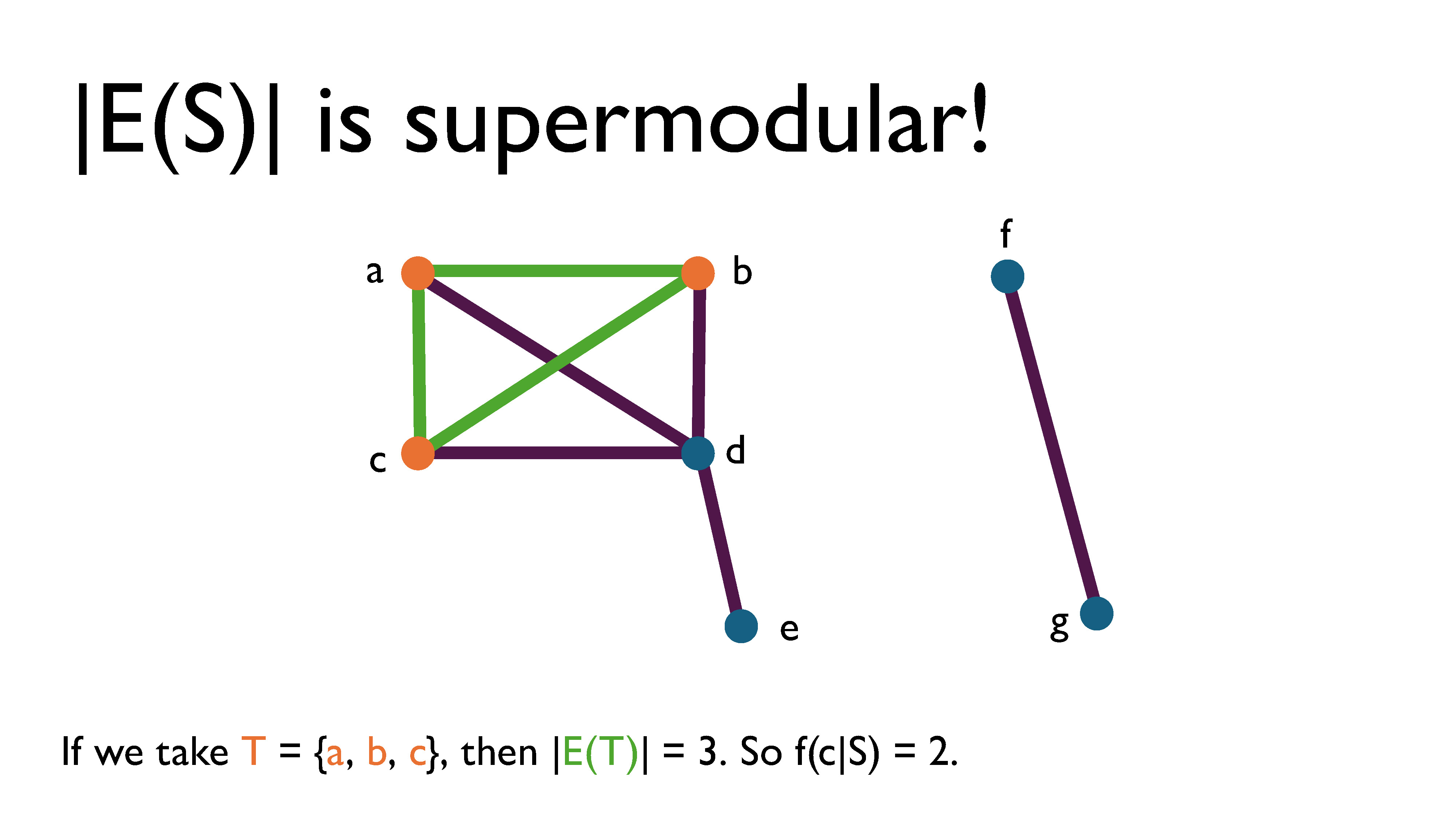
If we take $T = \{a, b, c\}$, then $|E(T)| = 3$. So $f(c|S) = 2$.

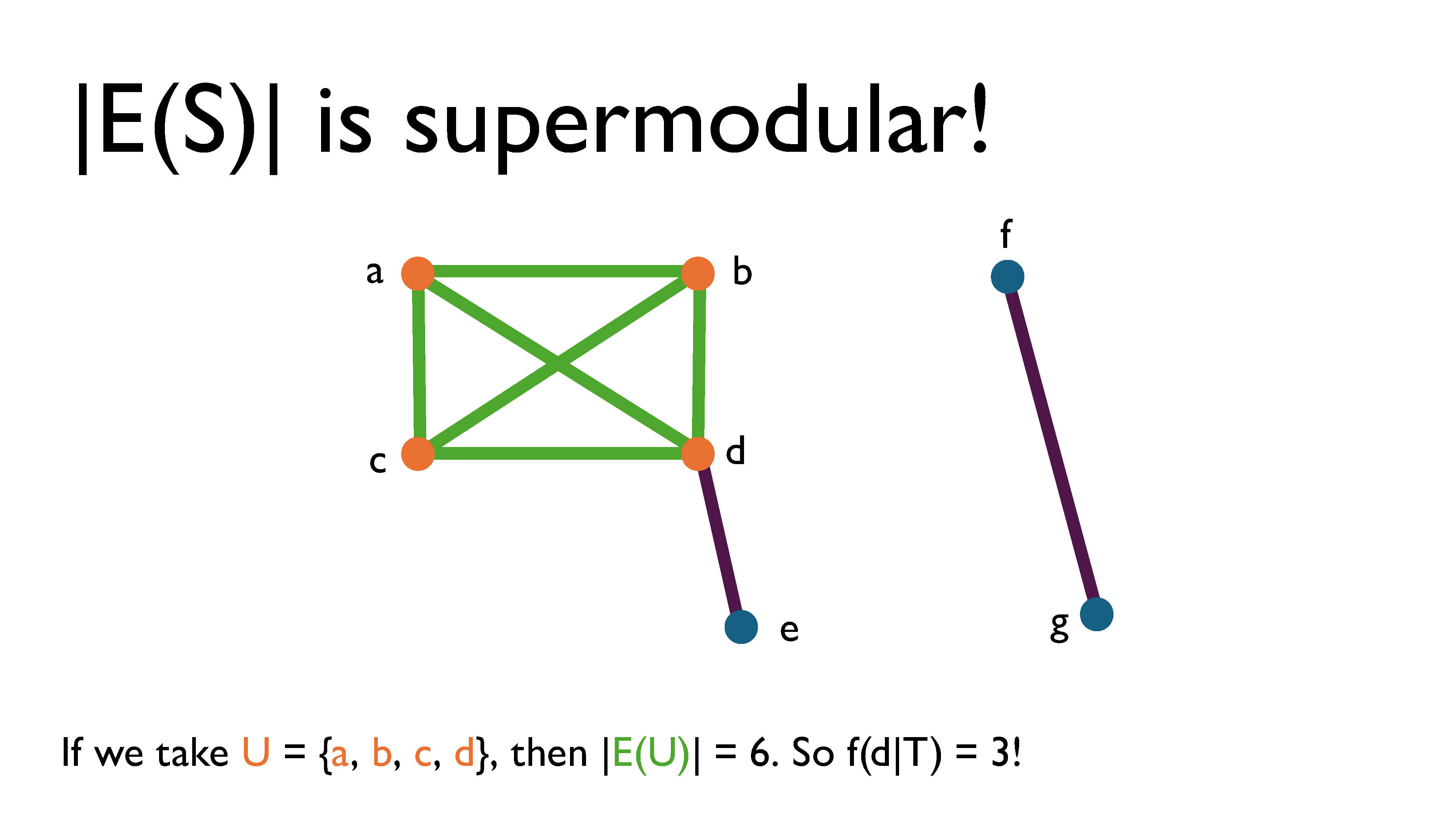
If we take $U = \{a, b, c, d\}$, then $|E(U)| = 6$. So $f(d|T) = 3$. This clearly shows that this function has increasing returns, which intuitively makes sense; the more vertices are in the subgraph, the more edges can be included in the induced graph by adding another vertex.

Subbing in $|E(S)|$ for $f(S)$ then, it’s clear that the DSP is a special case of the DSSP.

Now, if we were somehow able to generalize iterative peeling to work for all supermodular set functions, then perhaps we could use it to solve a lot more problems than just the DSP. Amazingly, this was shown to work by Charikar, Quanrud, and Torres in their 2022 paper (link here). They called the iterative peeling algorithm for supermodular set functions SuperGreedy++².

In general, for supermodular set functions, we just peel based on the marginal values of elements to the current set instead of peeling based on the degree of a vertex. (In fact, if our function is $|E(S)|$, then the current degree of some vertex $v$ in $S$ is actually its marginal value to $S$). Everything else about peeling stays the same.

Iterative peeling works for any set with a supermodular function. Chekuri, Quanrud, and Torres also showed that SuperGreedy++ is a $(1-\epsilon)$–approximation to the DSSP. What this means, very roughly, is that you can get as close as you want to the optimal answer so long as you’re willing to run enough iterations (and the number of iterations required depends on how small you decide your error tolerance is). This also tells us that it’s a $(1-\epsilon)$–approximation to the DSP.

Key Takeaways

So what did we learn from all of this? There were many detours, but overall, I hope you were able to get a sense of how we can use theoretical approaches to come up with solutions to problems.

There are three main things I’d like you to take away from this series:

1. Theory is useful because it helps us develop language to describe problems more precisely.
2. Theory helps us understand how different problems are related, through the use of abstraction.
3. Theory helps us find ways to reuse existing solutions or approaches, through the use of generalization.

Lastly, I hope you gained a little bit more of an appreciation for math³. I know I may have lost some of you part of the way through the formalism and minutiae, and that’s okay. But I hope you understand that these abstractions aren’t just some pointless thing mathematicians make us learn to make their field seem more legitimate. They can actually be useful in concrete ways, sometimes⁴.

This the last official segment of my series of writeups of this talk I did on a whim several months ago. If you’ve read all four of the articles, thank you!! It means a lot to me.

Serializing this series is the only reason it got done at all – without the pressure of having the previous articles out there and wanting to have a complete set, I don’t know that I ever would have finished this. So if you’re like me and disliked having unfinished projects out in the wild, maybe consider incremental release as a motivator for eventually getting the whole thing done⁵.

If for some reason, you did want more, there will be two more segments: one with resources and further reading (available here), and another on the writing (creating?) of this talk and series.