Why Does Theory Matter in Computer Science? /

Why Does Theory Matter in Computer Science? (Part 3)

The Densest Subgraph Problem, Peeling, and Iterative Peeling Algorithms

• February 13, 2025
• talks  
• notes  
• math  
• computer science  
• explainers  
• graph theory  
• algorithms  

This is the third installment in the written version of my talk about why I think theory matters in computer science. You can find part 2 here and the entire series is archived here. Stay tuned for part 4!

Abstraction: The Densest Subgraph Problem (DSP)

In Part 2 of this talk, we gave a crash course to graph theory and showed how we can use it to view some real-world problems as instances of the densest subgraph problem (DSP). But what exactly is the DSP?

If you’ve studied graph theory, you may have heard of something called the Maximum Clique Problem. The goal of the max clique problem is to find the largest complete subgraph in a graph. If we consider our vertices to be people, and edges to represent a friendship relationship between two people, in the max clique problem we are trying to find the largest friend group in a community. This is a famously difficult problem – it is NP-Hard, meaning that we strongly believe that creating an algorithm that does this efficiently is impossible.

The DSP can be viewed as a loose extension of the max clique problem: in this case, we are trying to find the subgraph with the highest average degree. Going back to our example, this means we want a group of people where on average, each person is friends with a large number of people. You could also see it as the group where “the most people know each other”, or as the group that maximizes the ratio of friendships to people.

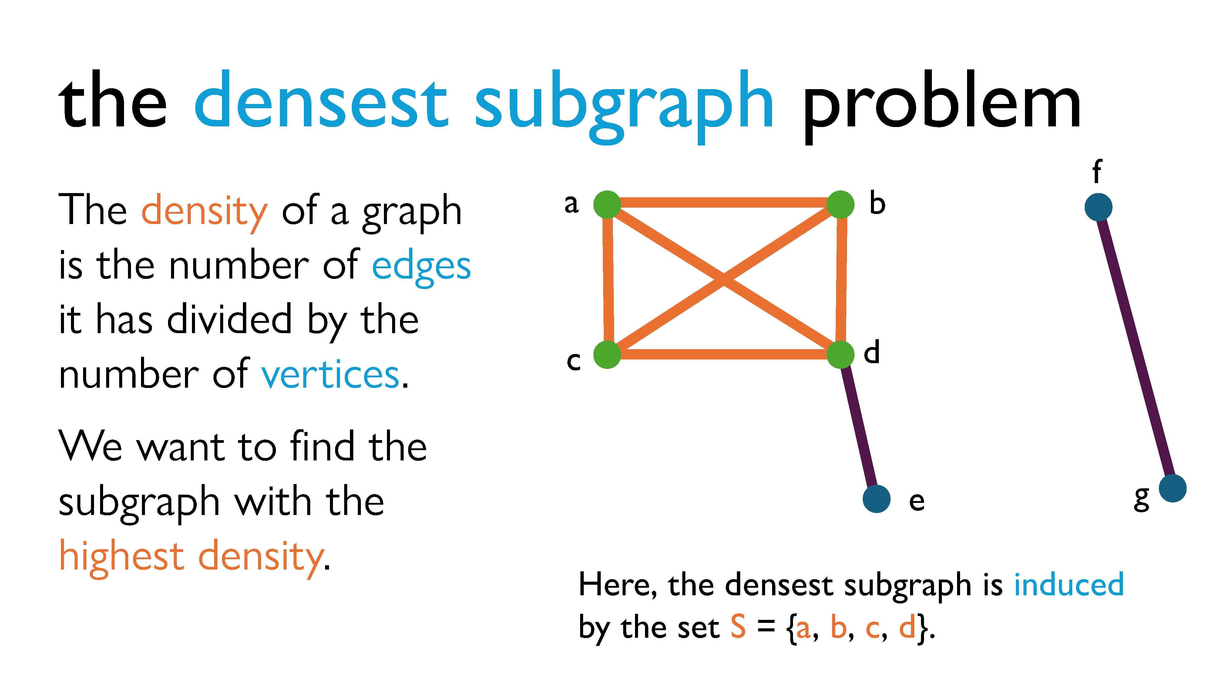
If we go back to looking at graphs more concretely, the density of a graph is usually defined by the number of edges it has divided by the number of vertices it has, and when solving the DSP we try to find the subgraph with the highest density. The term “density” comes from the idea of finding a subgraph that maximizes some ratio with respect to the properties of the graph. Usually, that property is the ratio of edges to vertices (aka relationships to objects), and that’s typically what we refer to when we talk about the DSP. (It’s also what we will focus on for now.) However, I should probably note that there are many variants of the DSP, which use all sort of other types of density measures.

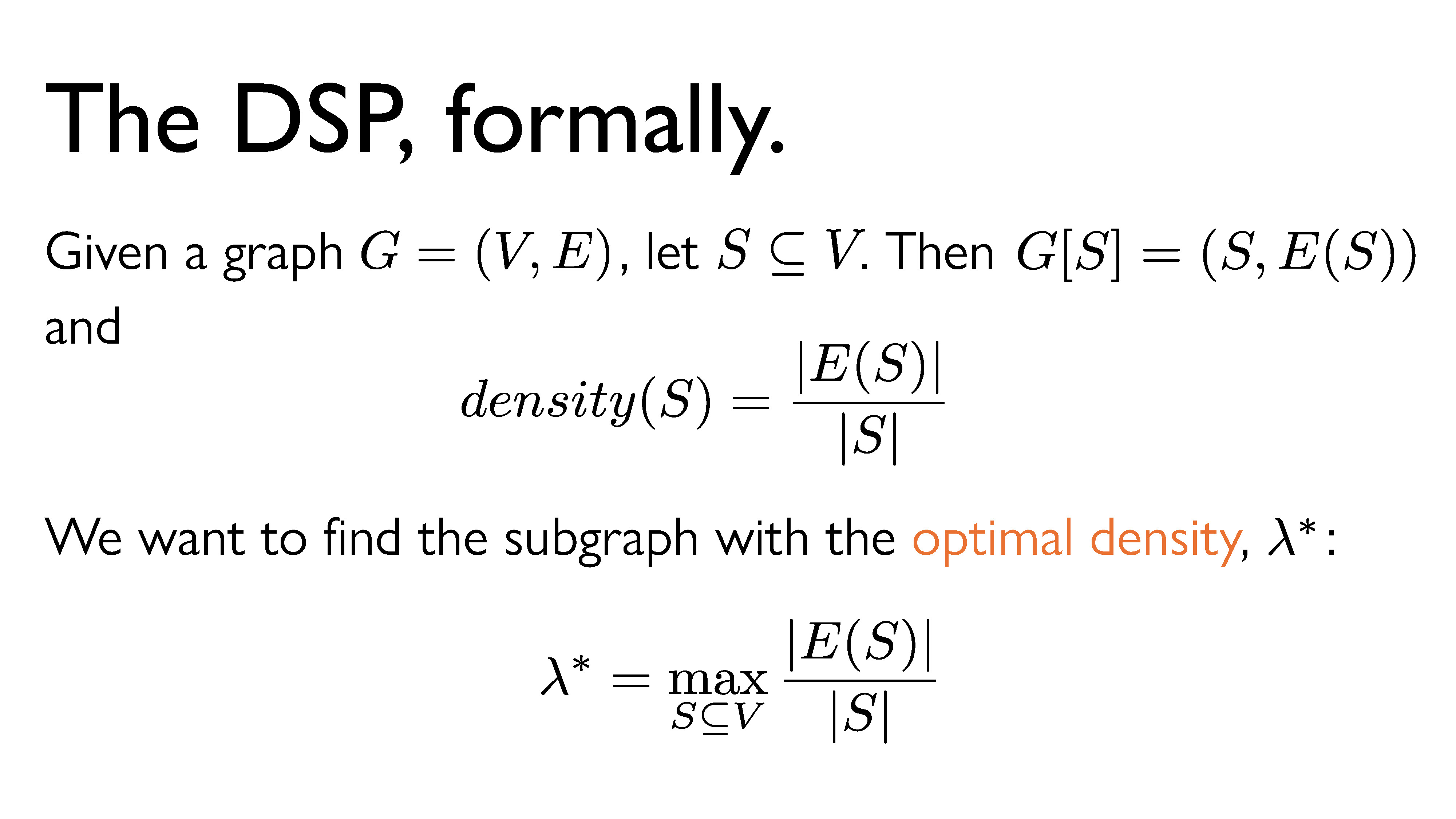
Here’s a more formal statement of the DSP: Given a graph $G = (V, E)$ , let $S$ be a subset of $V$ (the vertex set of $G$). We define $density(S)$ (the density of the subgraph induced by S) to be $|E(S)|$ (the number of edges in the induced graph) divided by $|S|$ (the number of vertices in $S$). We want to find the subset that maximizes the density, and we’re going to call that density the optimal density and denote it $\lambda^*$.

Approximation Algorithms for the DSP

Now that we’re clear on what exactly the DSP is, we need algorithms that solve it for us. We have algorithms that always find the correct densest subgraph with the optimal density, but they are… not great. In theory, we can find exact solutions to this problem efficiently (that is, in polynomial time), but in practice, the algorithms that are meant to do that eat up way too much memory and never terminate.

So, we’re going to look at some sketchier algorithms today – algorithms that give us “reasonable” or “good enough” candidates for the optimal subgraph. An algorithm that gives us a reasonable answer with some sort of guarantee on the “quality” of the solution found is called an approximation algorithm (I’ve written more on those here), and we’ll mainly be looking at two of them here.

Peeling

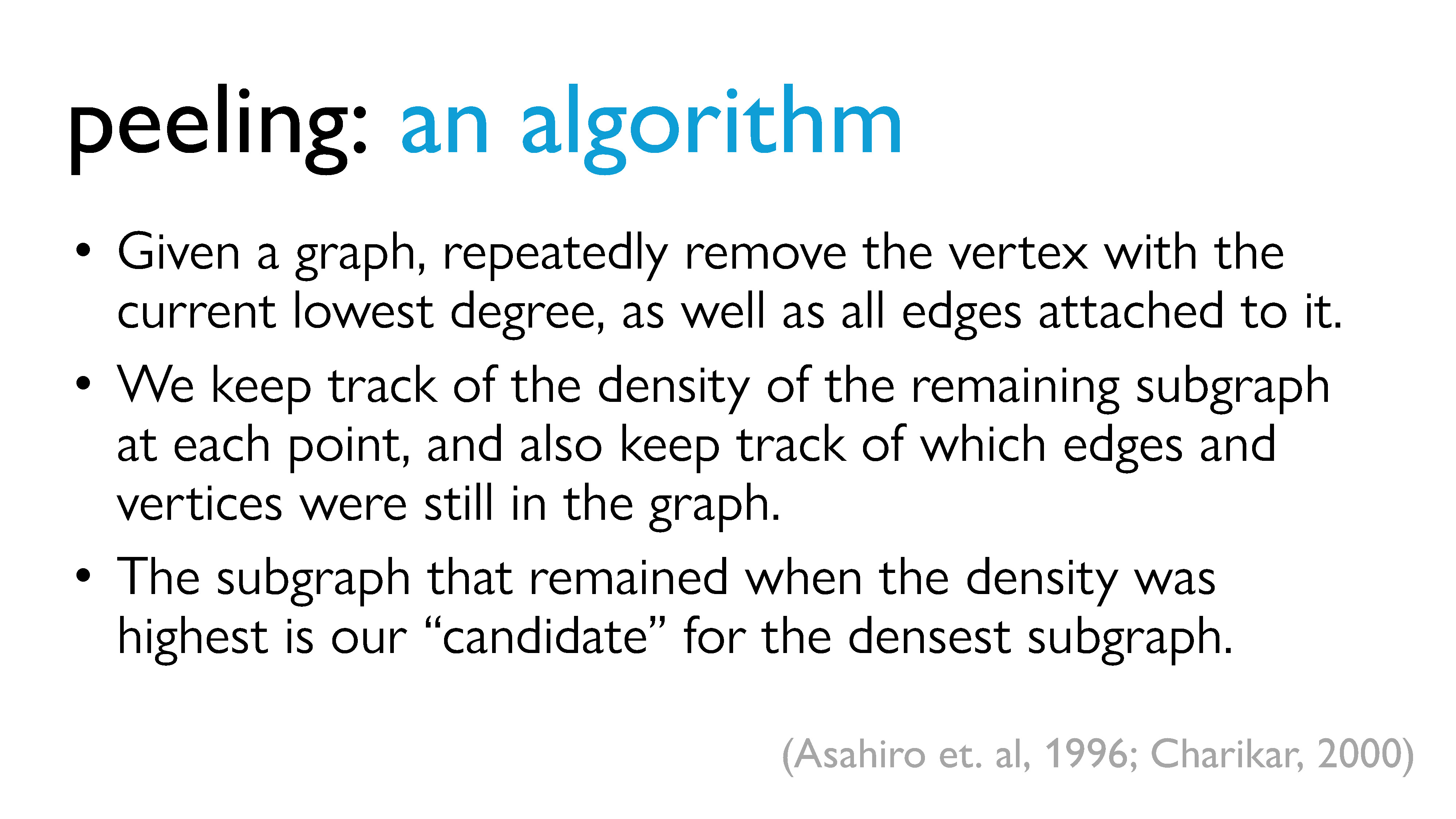
The first algorithm we’re going to look at is called peeling¹, which dates back to around the year 2000 and is actually used in the real world. The idea is that we peel away vertices of low degree: this means that at each peeling step, we remove the vertex with the lowest degree, as well as all of the edges that are attached to it. As we continue to peel vertices, the density of the graph changes – at some points it may increase, and at other points it may decrease. We keep track of the density of the graph at every point, and the point in our peeling at which the density was highest is our “candidate” for the densest subgraph.

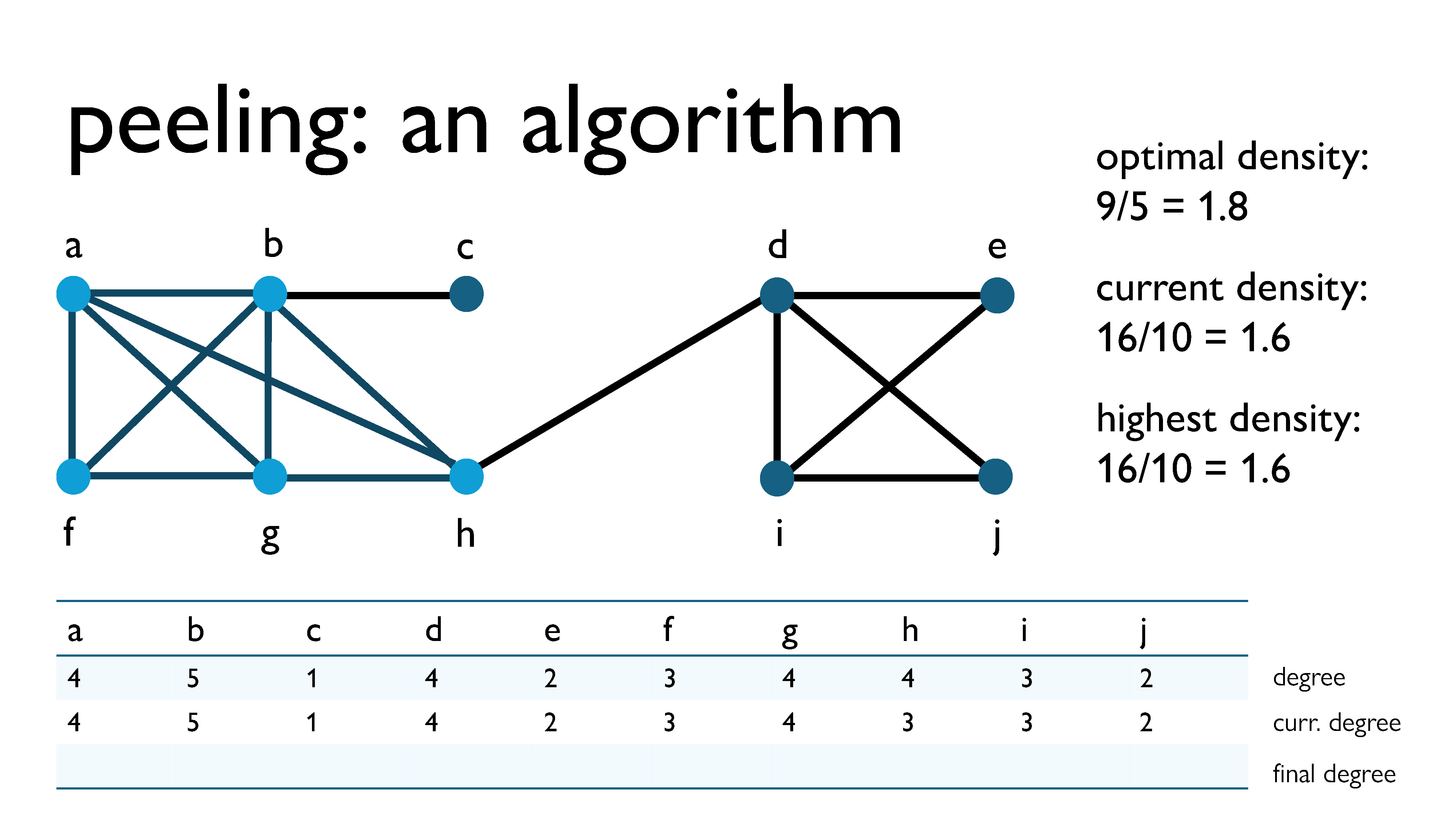
Here’s an example graph I’m going to use to demonstrate the peeling process. The part of the subgraph that is highlighted in blue is the actual densest subgraph, which I manually computed in advance. I’ve also put a table at the bottom of the slide, where you can see what the degrees of the vertices are as we peel them away, as well as some information about the density of the graph on the side. I’m going to peel away the vertices, and then we’re going to see which candidate the algorithm gives us for the densest subgraph.

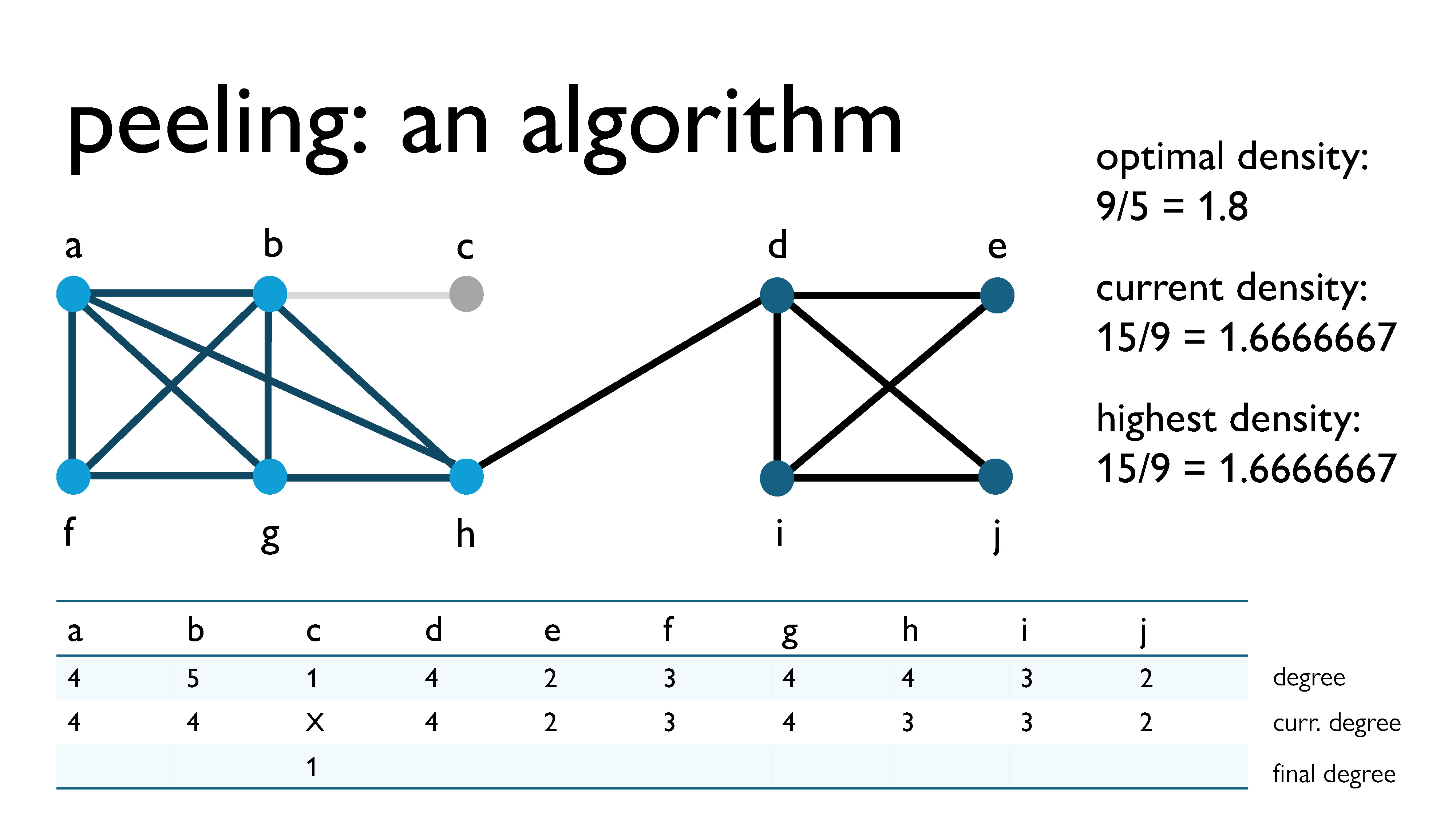
First, we peel vertex $c$, because it has the lowest current degree ($\text{curr\_deg}(c) = 1$). This now becomes its final degree.

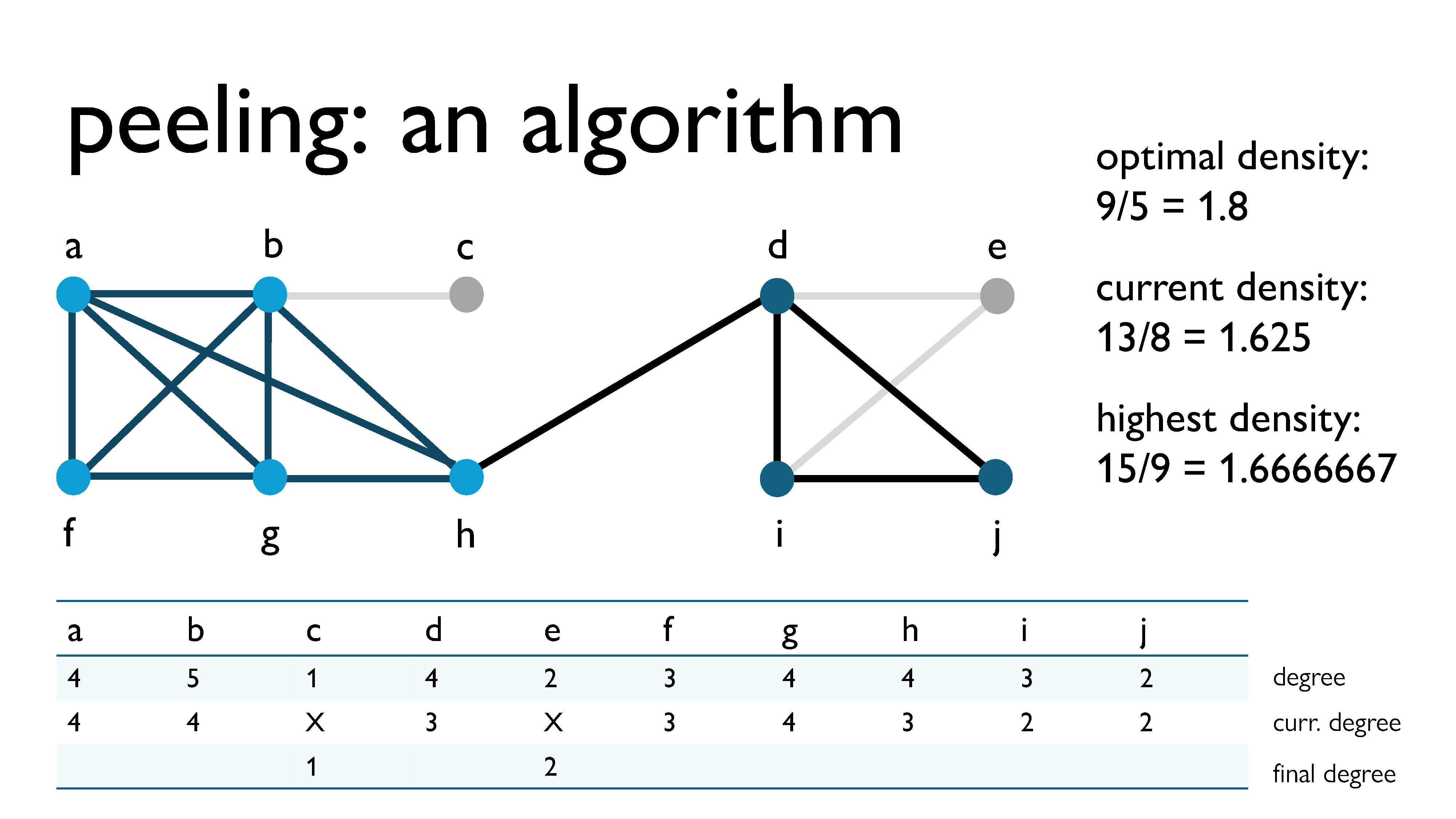
Then, we peel vertex $e$, because it has the lowest current degree ($\text{curr\_deg}(e) = 2$). This now becomes its final degree.

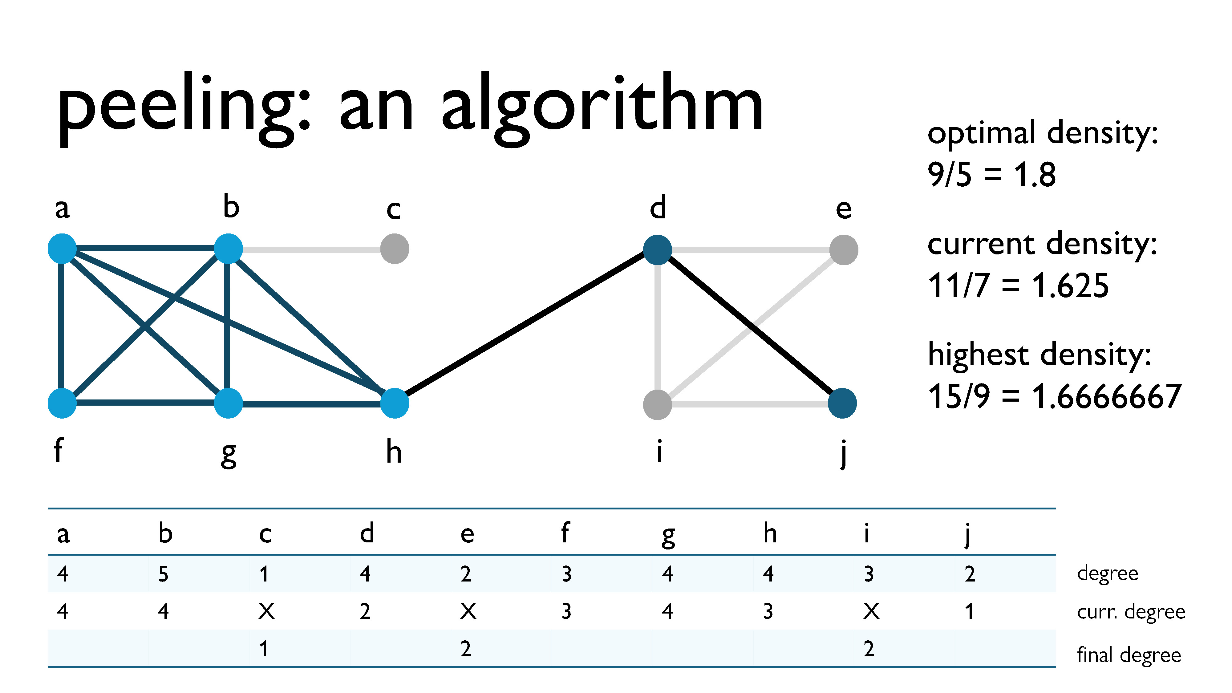
We repeat this process with all of the other vertices. Here, we’re peeling vertex $i$, with a current degree of 2.

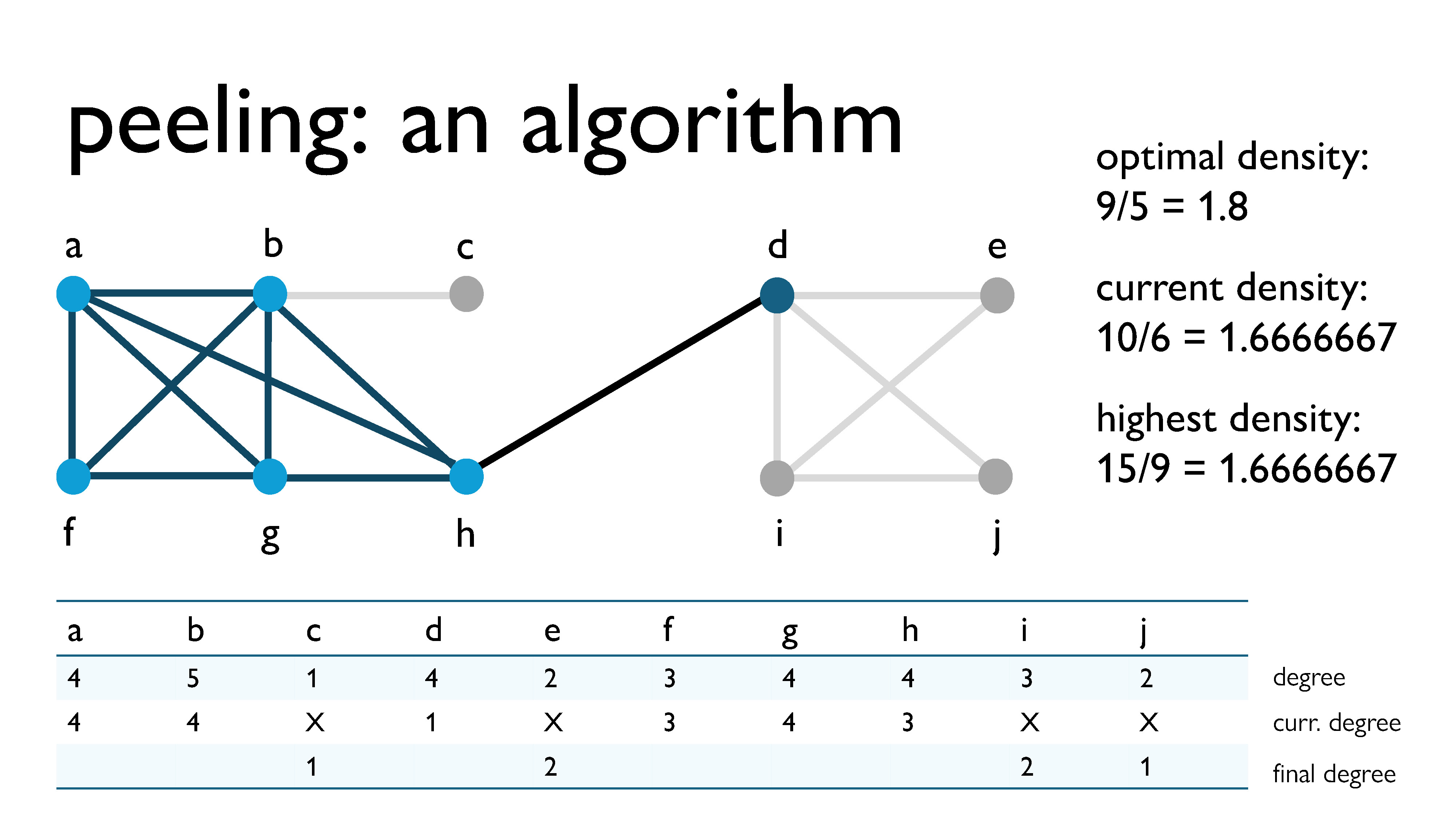
Here, we’re peeling vertex $j$, with a current degree of 1.

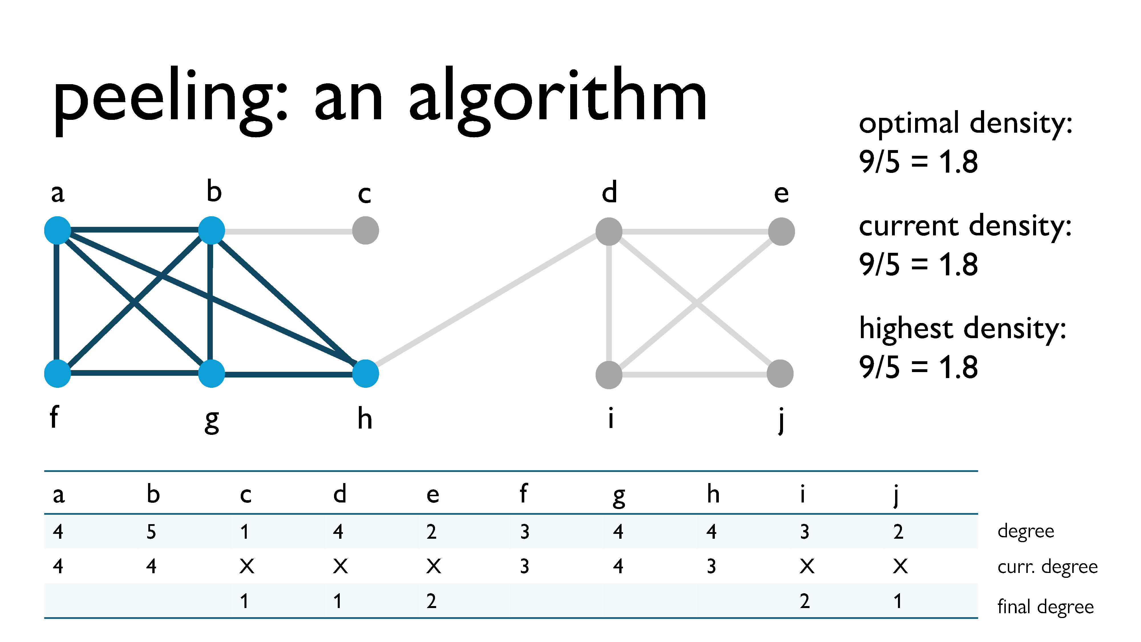
Here, we’re peeling vertex $d$, with a current degree of 1.

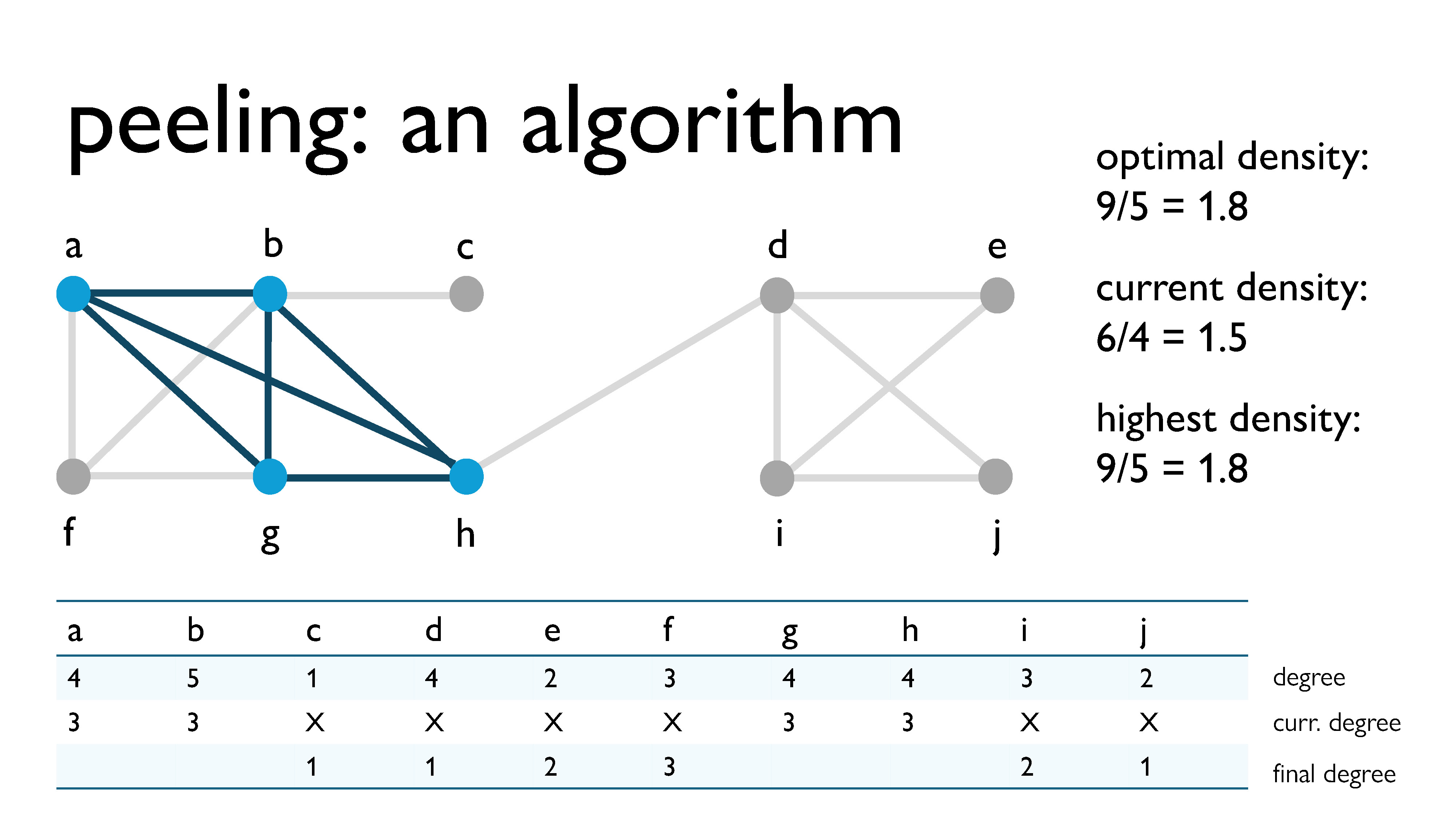
Here, we’re peeling vertex $f$, with a current degree of 3.

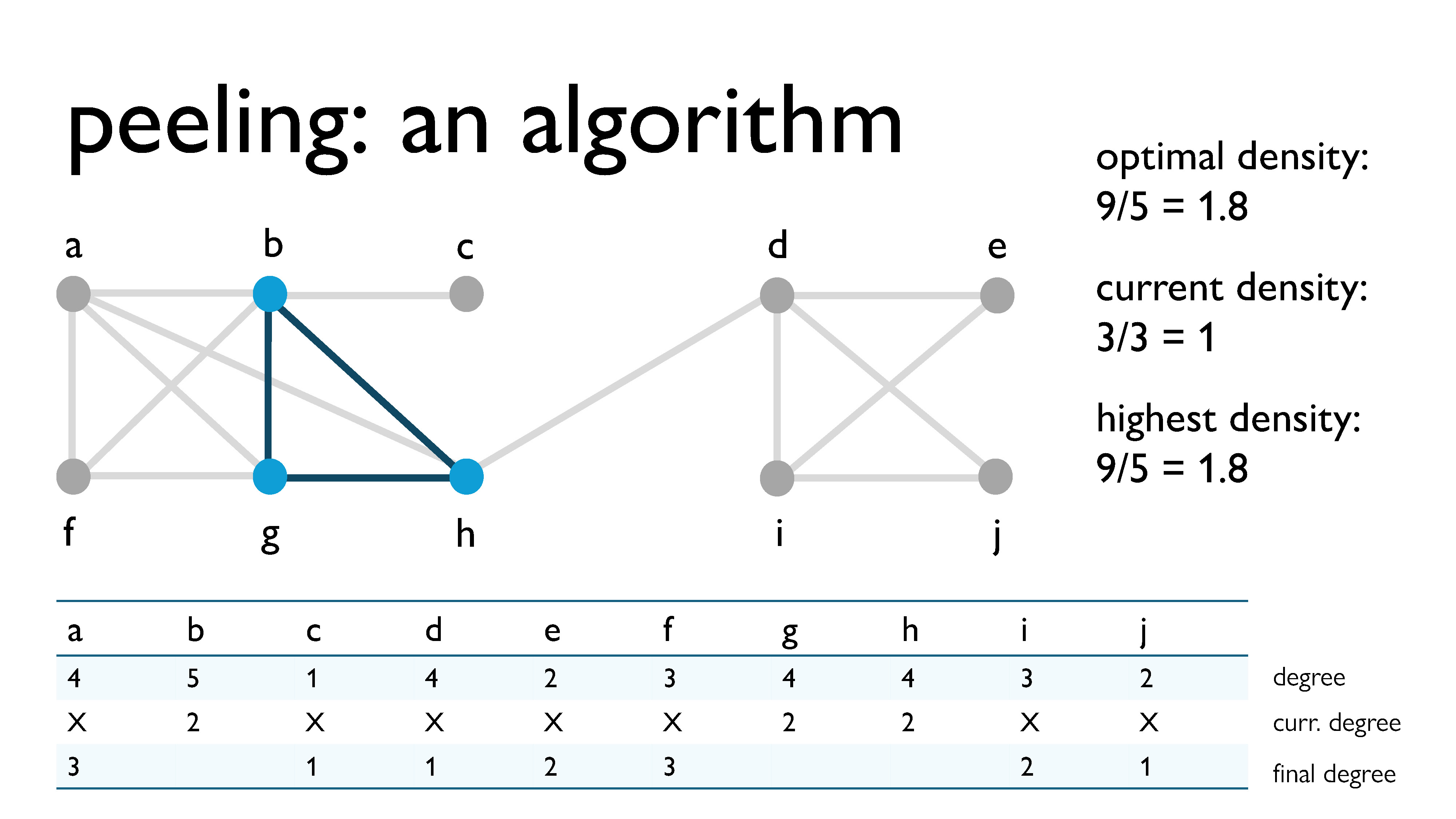
Here, we’re peeling vertex $a$, with a current degree of 3.

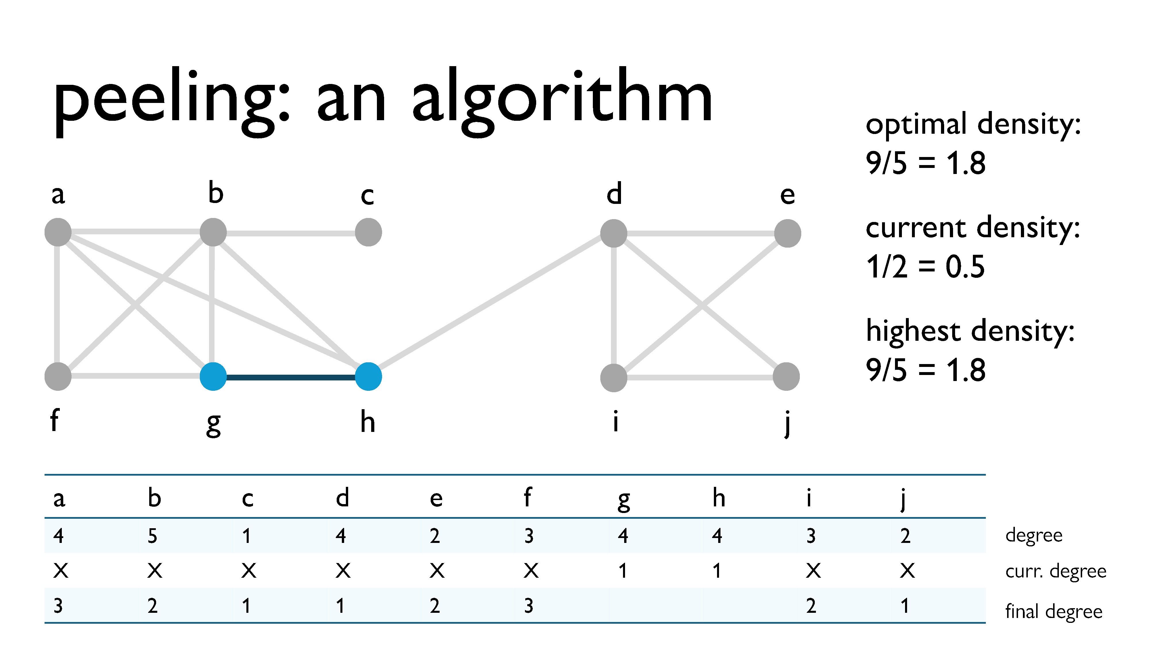
Here, we’re peeling vertex $b$, with a current degree of 2.

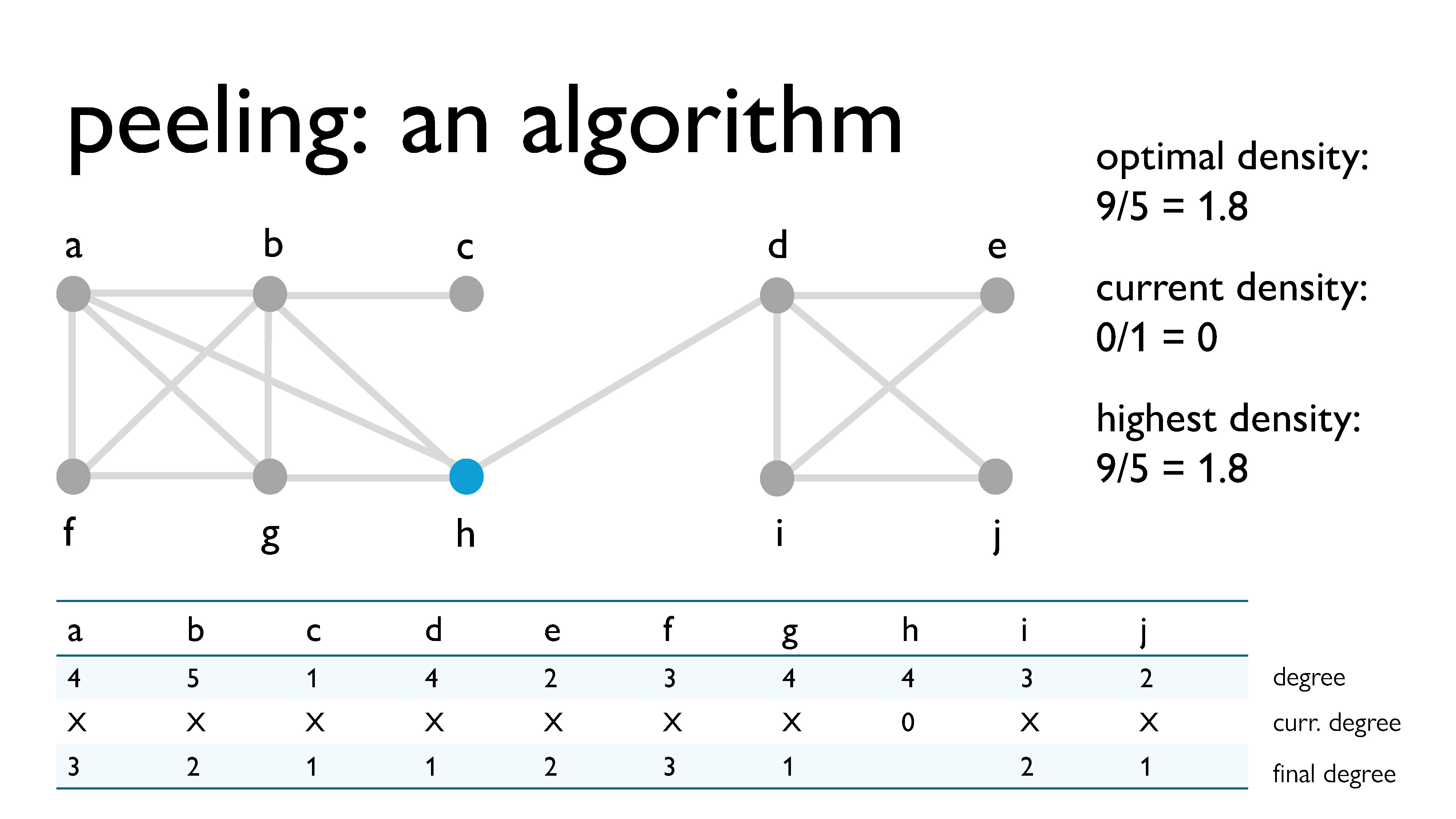
Here, we’re peeling vertex $g$, with a current degree of 1.

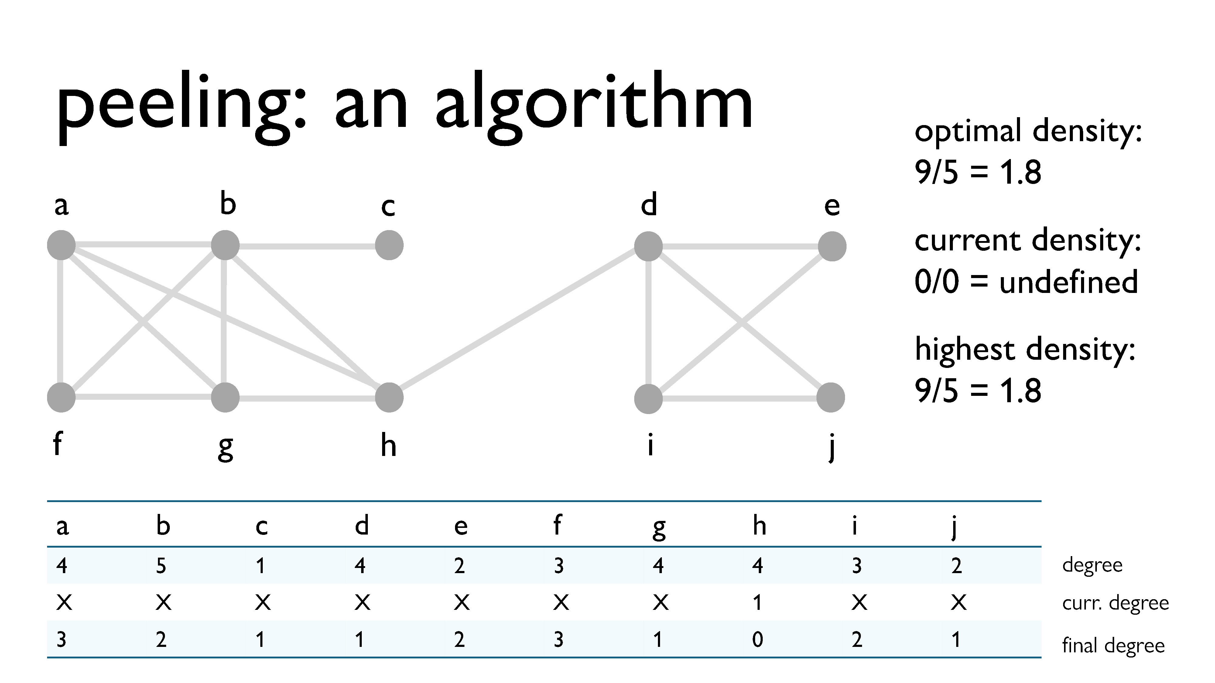
Finally, we peel vertex $h$, with a current degree of 0.

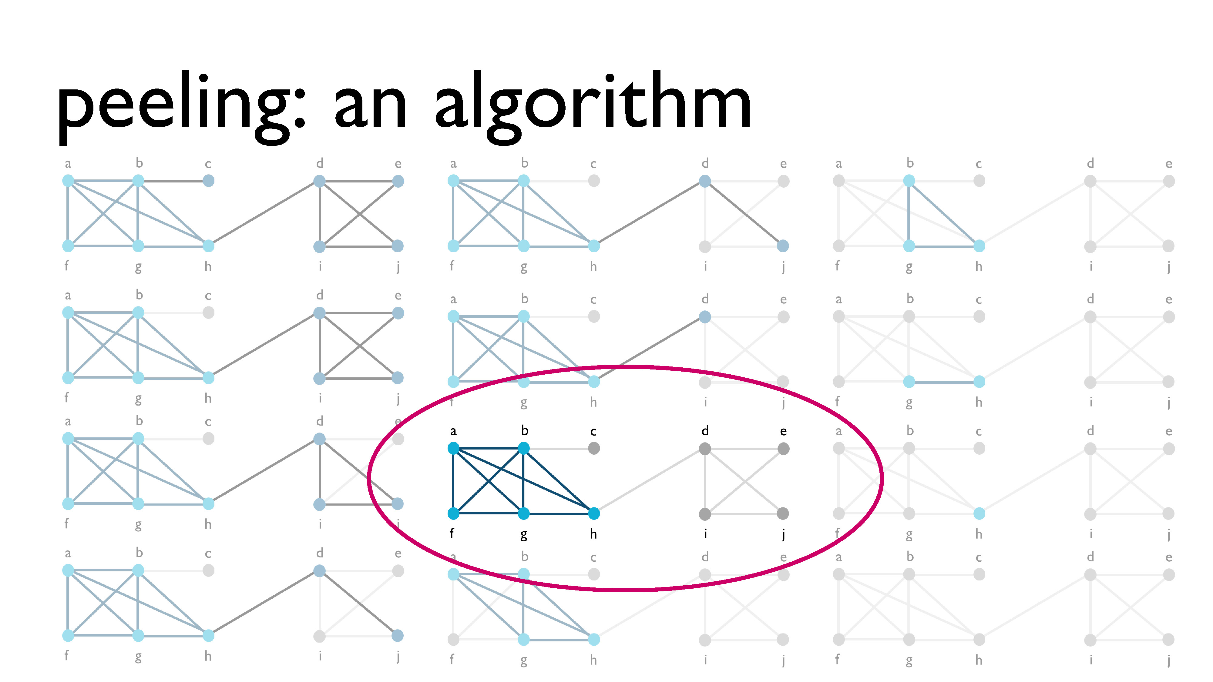
Now that we’ve peeled all of the vertices, we look back at all of the different subgraphs we had over the course of the process, and we choose the subgraph with the highest density, which is what you see circled here in pink.

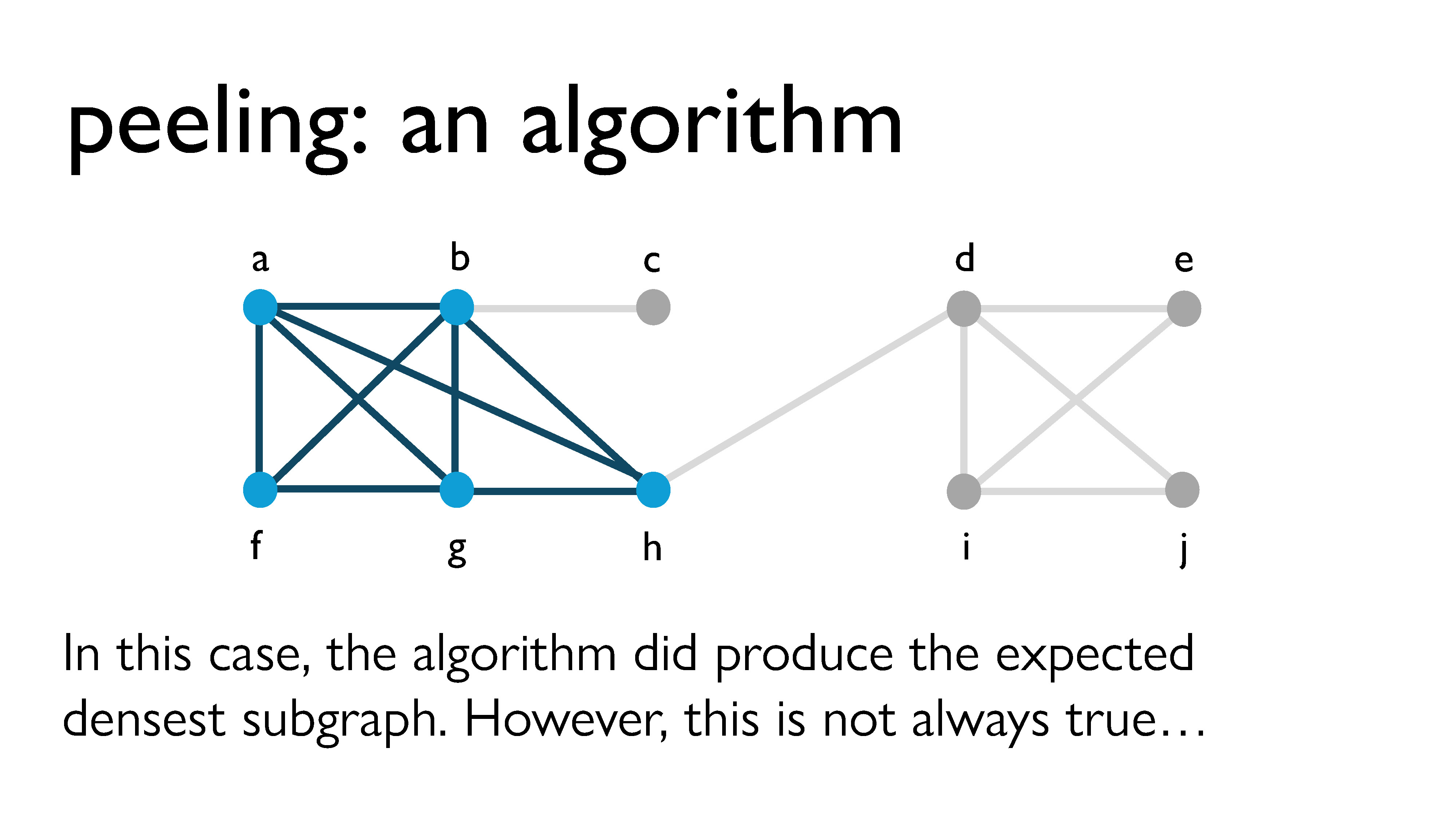
In this case, peeling did produce the correct densest subgraph. But it doesn’t always work exactly. In fact, peeling usually doesn’t quite work.

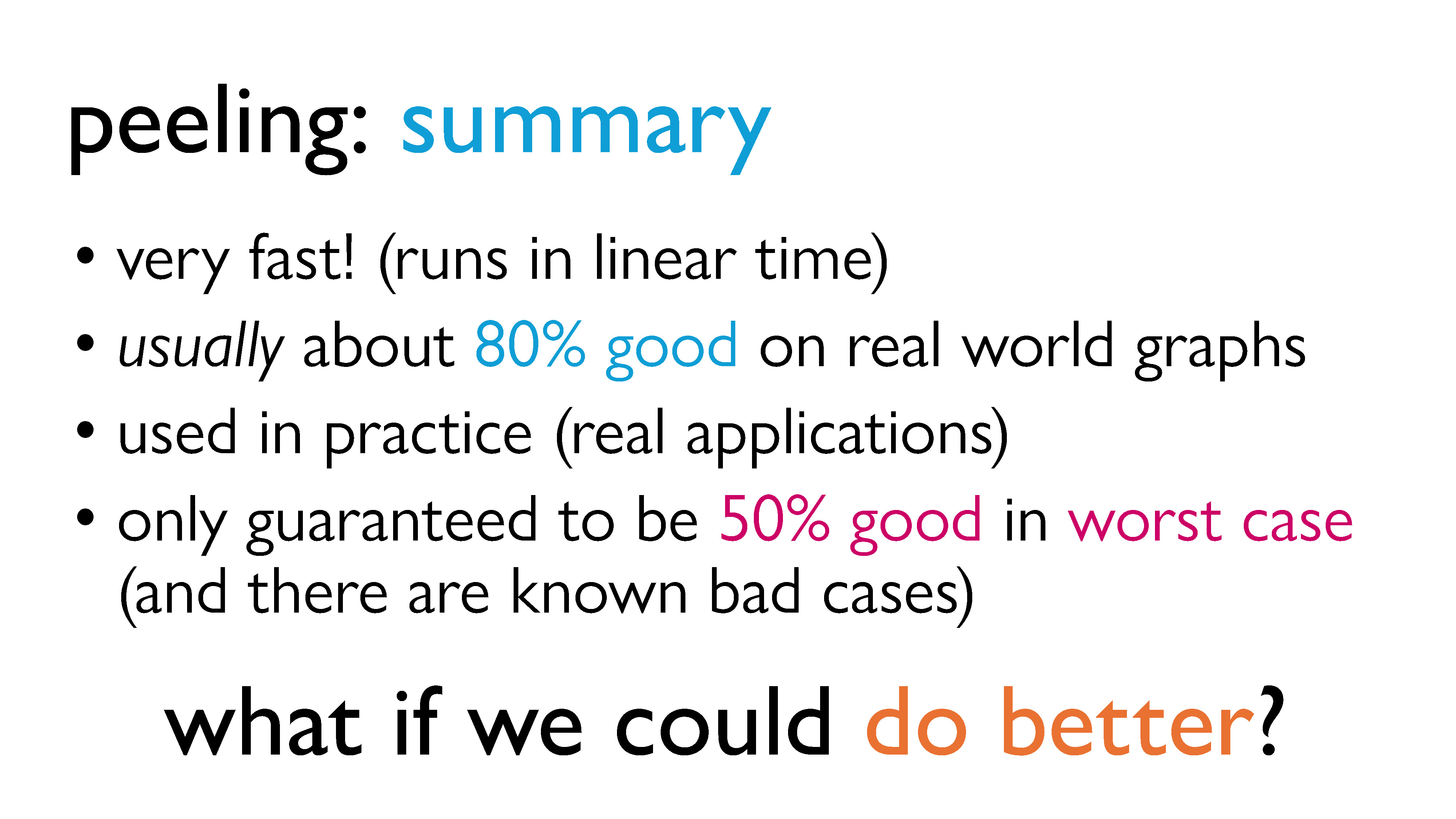
If we summarize our results from peeling, it is very fast! It runs in linear time. Usually, the graph it produces is about 80% as good as the actual densest subgraph. For a linear time algorithm, this is great, which is why it’s actually used in practice. However, it’s only guaranteed to be around 50%, and there are known “bad graphs” where that bound is tight. So what if 50% isn’t good enough for me? Can we do any better? This is where the idea of iterative peeling comes in.

Iterative Peeling

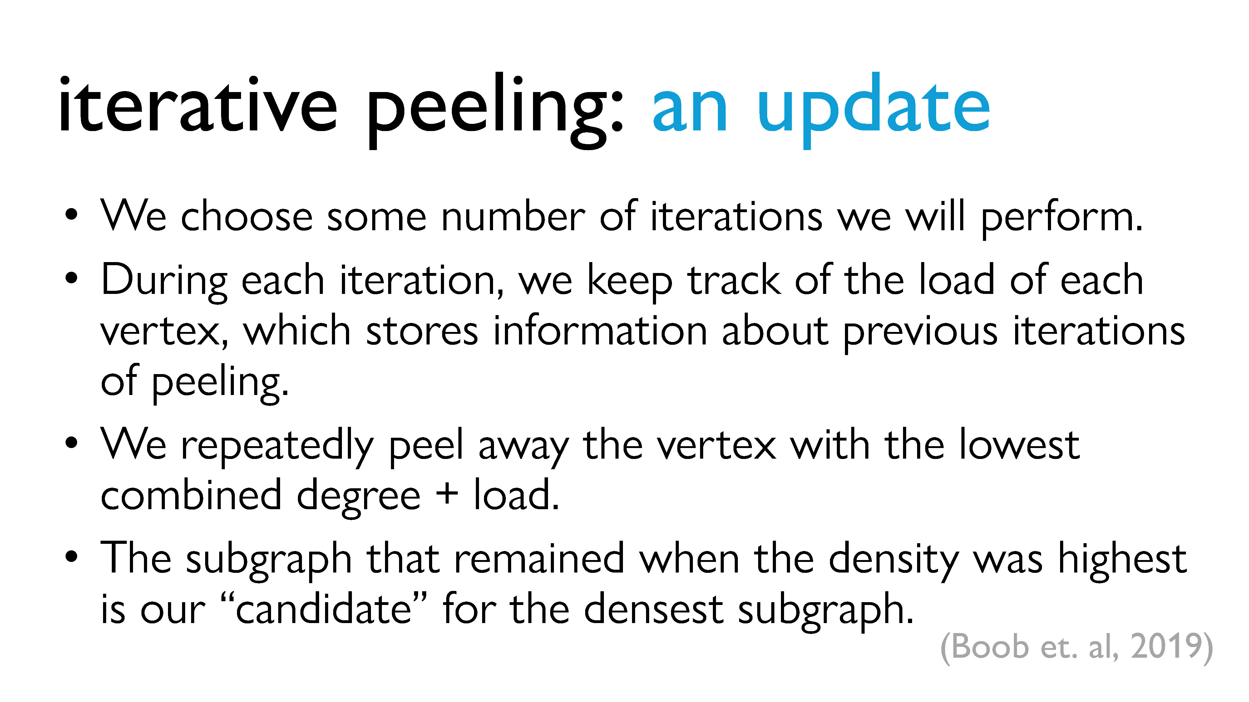
In around 2019, some researchers proposed that one way to improve the accuracy of our approximation could be to just repeat this peeling procedure over and over. The idea is that we first decide on the number of peeling iterations we are going to perform, where one iteration is a full cycle of peeling. During each iteration, in additional to keeping track of the current degree of each vertex, we keep track of a new piece of information called the load, which more or less stores information about the previous iterations. Instead of peeling based on the degrees of the vertices, we repeatedly peel away the vertex with the lowest combined current degree + load. Again, at each point, we keep track of the remaining subgraph, and the subgraph with the highest density becomes our candidate for the densest subgraph.

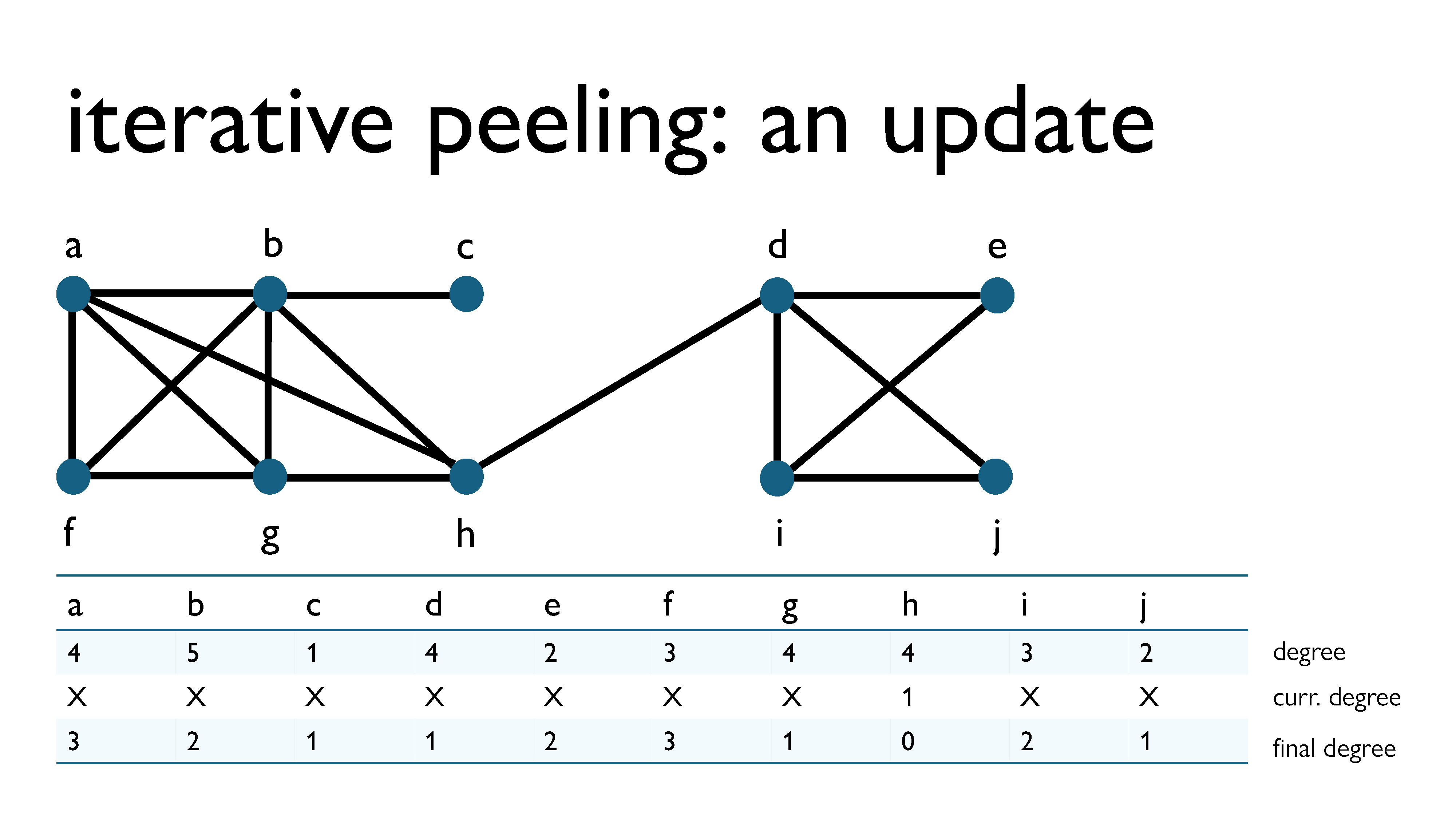
So how does this work? The first iteration of iterative peeling is exactly the same as a cycle of regular peeling, since we initialize the loads of all of the vertices to zero. So, let’s pick up from where we left off in the earlier peeling example. As you can see in the image above, in the previous example, we kept track of the degree of every vertex at the time when it was removed. You may have noticed me keeping track of this, and not known why. However, the degree at the time of removal gets added to the load of the vertex at the end of every iteration.

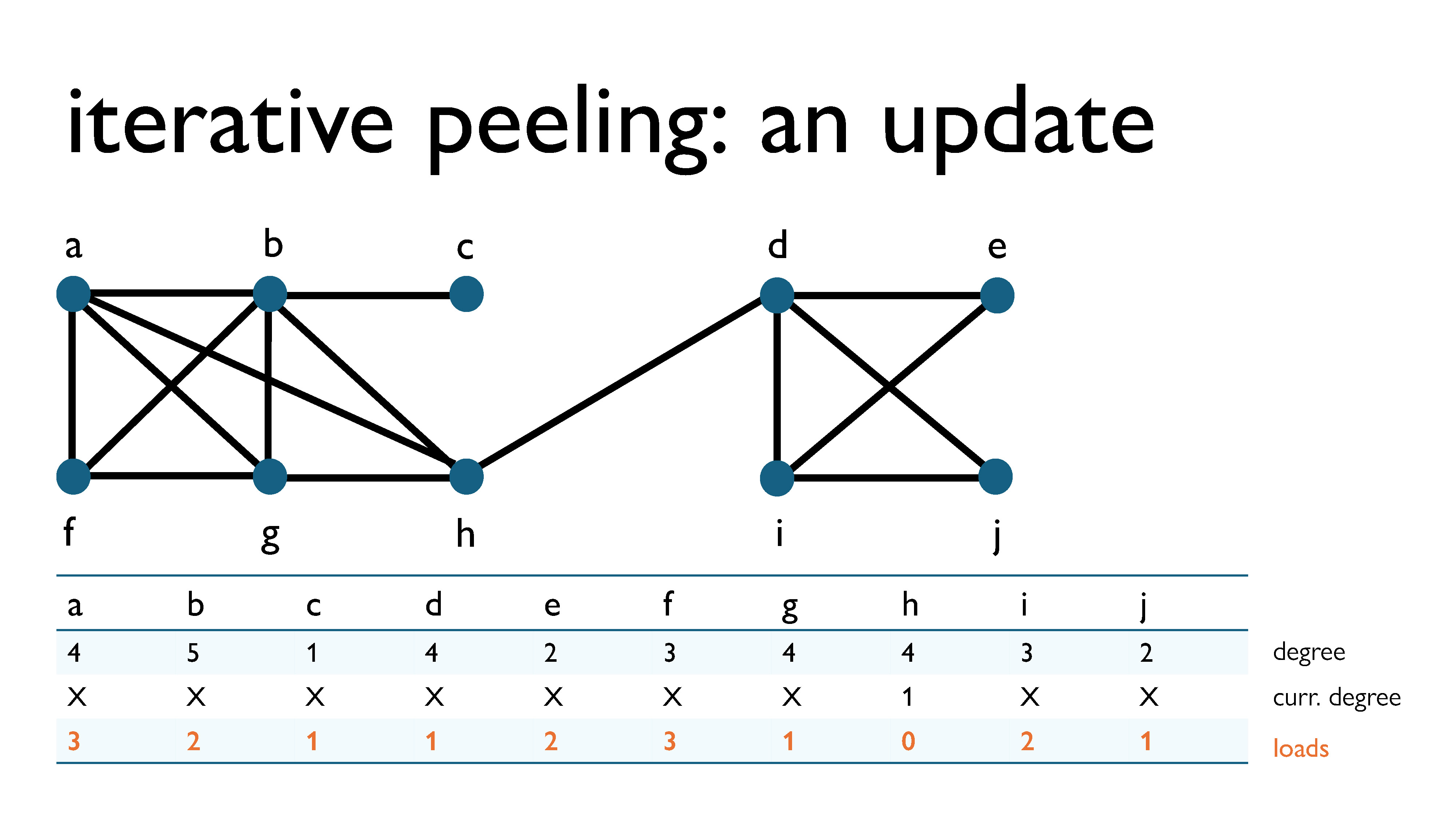
Since the load before the first iteration was 0 for each vertex, the load of each vertex after the first iteration will be equal to its degree at the time of removal.

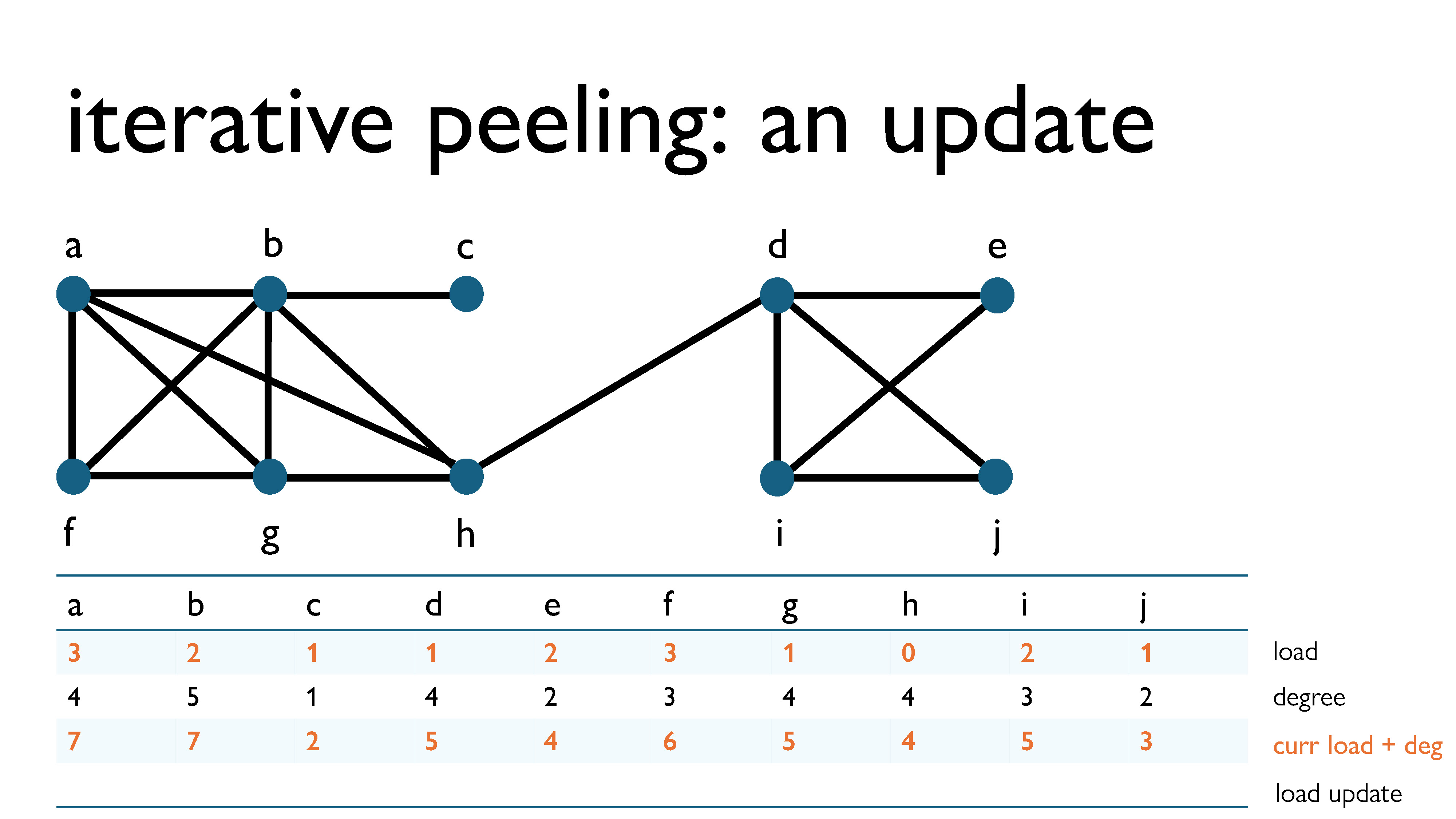
We can now update this diagram to keep track of loads, degrees, the current load + deg, and the load update (the value that will be added to the load after this iteration).

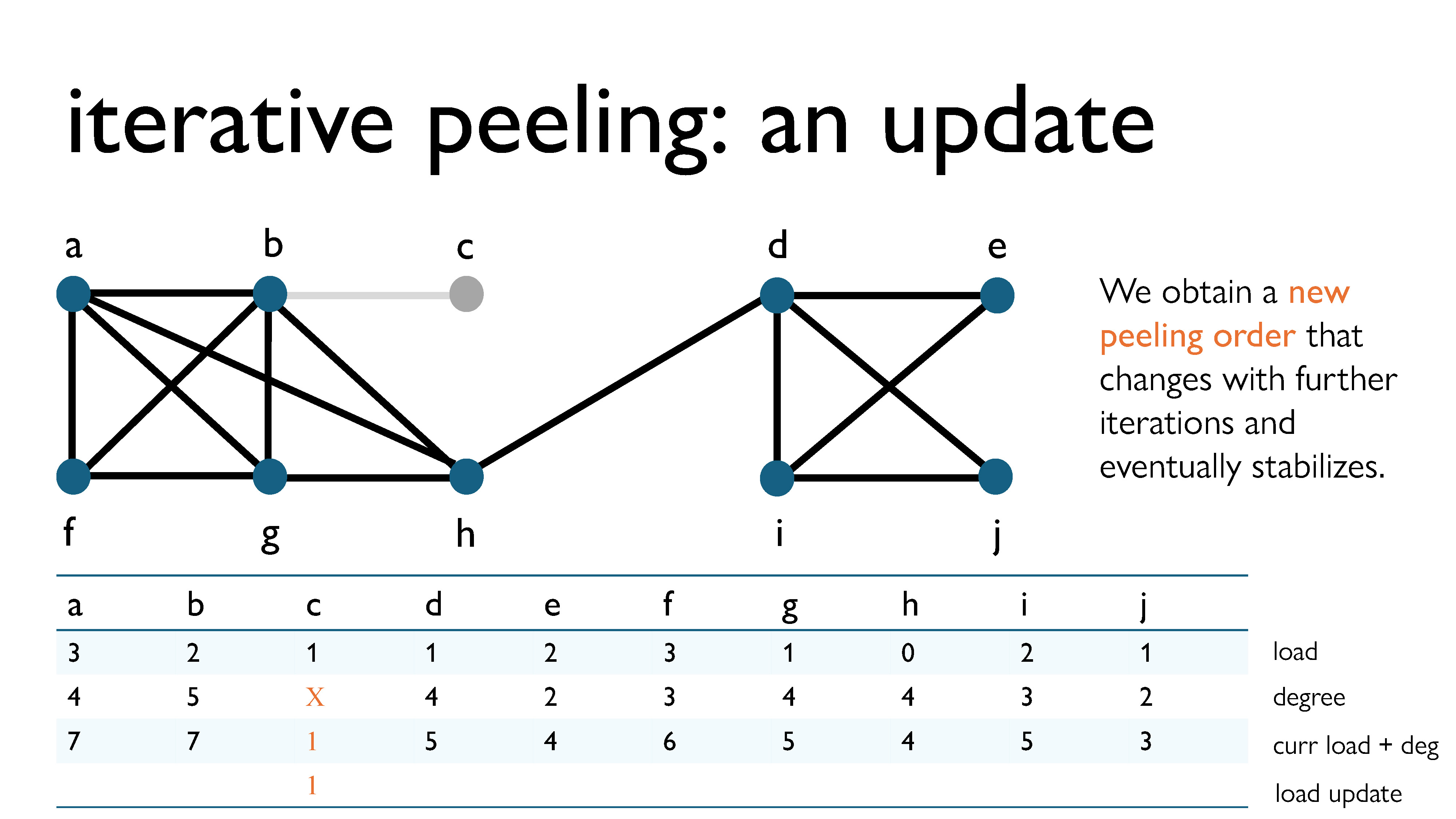
Here’s the first peeling step. We removed vertex c, since it had the lowest load + current degree in the graph. Since it had degree 1 at the time of removal, in the next iteration it will have load 1 (its current load) + 2 (its degree when removed) = 2.

What’s interesting is that with this new technique, the peeling order will begin to evolve with each iteration, and eventually, with enough iterations, it should stabilize itself.

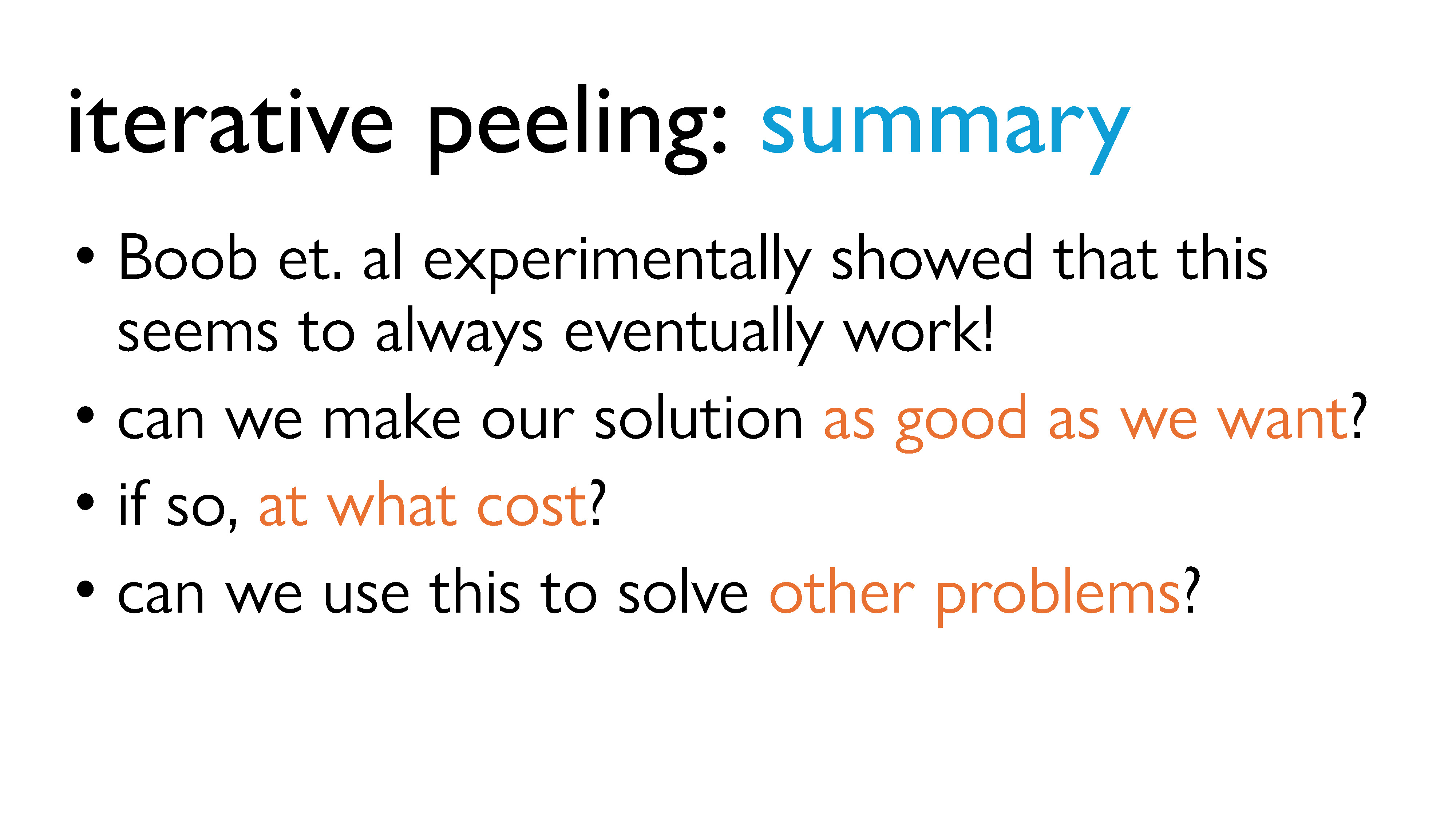
As you’ve probably noticed, it seems like if we do this procedure enough times, we’re always eventually going to get the optimal subgraph. But we don’t know if this is actually true, right? We hope it is, but we don’t really have a way to prove this right now. Also, this is a really simple procedure; like, it’s relatively simple to implement (which I actually spent a summer doing) and I could probably explain it to a ten-year old. So it would be really nice if we could use this method to solve other problems.

So it turns out that we can actually can answer these questions. We’re going to generalize a little bit, and do a bit more abstraction, but it is doable. We’ll look more into that in Part 4.